A New Ecology - Systems Perspective - Chapter 5 doc

5
Ecosystems have connectivity
“Life did not take over the globe by combat, but by networking.”
(Margulis and Sagan. Microcosmos)
5.1 INTRODUCTION
The web of life is an appropriate metaphor for living systems, whether they are ecological,
anthropological, sociological, or some integrated combination—as most on Earth now are.
This phrase immediately conjures up the image of interactions and connectedness both
proximate and distal: a complex network of interacting parts, each playing off one
another, providing constraints and opportunities for future behavior, where the whole is
greater than the sum of the parts. Networks: the term that has received much attention
recently due to such common applications as the Internet, “Six Degrees of Separation”,
terrorist networks, epidemiology, even MySpace
®
, actually has a long research history in
ecology dating to at least Darwin’s entangled bank a century and a half ago, through the
rise of systems ecology of the 1950s, to the biogeochemical cycling models of the 1970s,
and the current focus on biodiversity, stability, and sustainability, which all use networks
and network concepts to some extent. It is appropriate that interconnected systems are
viewed as networks because of the powerful exploratory advantage one has when
employing the tools of network analysis: graph theory, matrix algebra, and simulation
modeling, to name a few.
Networks are comprised of a set of objects with direct transaction (couplings) between
these objects. Although the exchange is a discrete transfer, these transactions viewed in
total link direct and indirect parts together in an interconnected web, giving rise to the net-
work structure. The structural relations that exist can outlast the individual parts that make
up the web, providing a pattern for life in which history and context are important. The
connectivity of nature has important impacts on both the objects within the network and
our attempts to understand it. If we ignore the web and look at individual unconnected
organisms, or even two populations pulled from the web, such as one-predator and one-
prey, we miss the system-level effects. For example, in a holistic investigation of the

Florida Everglades, Bondavalli and Ulanowicz (1999) showed that the American alligator
(Alligator mississippiensis) has a mutualistic relation with several of its prey items, such
that influence of the network trumps the direct, observable act of predation. The connected
web of interactions makes this so because each isolated act of predation links together the
entire system, such that indirect effects—those mitigated through one or many other
objects in the network—can dictate overall relations. While this might seem irrelevant par-
ticularly for the individual organisms that end up in the alligator’s gut, as a whole the prey
79
Else_SP-Jorgensen_ch005.qxd 4/12/2007 17:45 Page 79
80
A New Ecology: Systems Perspective
population benefits from the presence of the alligator in the web since it also feeds on
other organisms in the web which in turn are predators or competitors with the prey.
Such discoveries are not possible without viewing the ecosystem as a connected net-
work. This chapter deals with that connectivity, provides an overview of systems
approaches, introduces quantitative methods of ecological network analysis (ENA) to
investigate this connectivity and ends with some of the general insight that has been
gained from viewing ecosystems as networks. Insight, which at first glance appears
surprising and unintuitive, is not that surprising under closer inspection. It only seems
so from our current paradigm, which is still largely reductionistic. We hope these
examples give further weight for adopting the systems perspective promoted through-
out this book.
5.2 ECOSYSTEMS AS NETWORKS
Ecosystems are conceptual and functional units of study that entail the ecological com-
munity together with its abiotic environment. Implicit in the concept of any system, such
as an ecosystem, is that of a system boundary which demarcates objects and processes
occurring within the system from those occurring outside the system. This inside–outside
perspective gives rise to two environments, the environment external to the system within
which it is embedded, and the environment outside the object of interest but within the
system boundaries (the latter has been termed environ by Patten, 1978). We typically

are not concerned with events occurring wholly outside the system boundary, i.e., those
originating and terminating in the environment without entering the system by crossing
the system boundary. Furthermore, as open systems, energy–matter fluxes occur across
the boundary; these in turn provide the ecosystem with an available source of energy input
such as solar radiation and a sink for waste heat. In addition to continuous radiative energy
input and output, pulse inputs are important in some ecosystems such as allochthonous
organic matter in streams and deltas, and migration in Tundra.
The spatial extent of an ecosystem varies greatly and depends often on the functional
processes within the ecosystem boundaries. O’Neill et al. (1986) defined an ecosystem
as the smallest unit which can persist in isolation with only its abiotic environment, but
this does not give an indication to the area encompassed by the ecosystem. Cousins
(1990) has proposed the home range or foraging range of the local dominant top preda-
tor arbiter of ecosystem size, which he refers to as an ecosystem trophic module or
ecotrophic module. Similar to the watershed approach in hydrology, Power and Rainey
(2000) proposed a “resource shed” to delineate the spatial extent of an ecosystem. Taken
to the extreme, one could eliminate environment altogether by expanding the boundaries
outward indefinitely to subsume all boundary flows, thus making the very concept of
environment a paradox (Gallopin, 1981). The idea is not to make the “resource shed” so
vast as to include everything in the system boundary, but to establish a demarcation line
based on gradients of interior and exterior activities. In fact, in open systems an external
reference state is a necessary condition, which frames the ecosystem of interest (Patten,
1978). We give the last word to Post et al. (2005) who stated that different organisms
within the ecosystem based on their resource needs and mobility will operate at different
Else_SP-Jorgensen_ch005.qxd 4/12/2007 17:45 Page 80
temporal and spatial scales, typically leaving the scale context-specific for the research
question in hand.
Definitional difficulties aside, one must operationalize an ecosystem so following
O’Neill’s approach of the smallest unit that could sustain life, the minimum set for a
sustainable functioning ecosystem comprises producers and consumers, specifically
decomposers (see further below). One visualizes a naturally occurring biotic community

to include:
(1) organisms that can draw in and fix external energy into the system, typically primary
producers,
(2) additional organisms that feed on this fixed energy, consumers, and
(3) decomposers that close the cycle on material flow as well as provide additional
energy pathways.
This biotic community interacts with its abiotic environment acquiring energy, nutrients,
water, and physical space to form its place or habitat niche (although habitat is often
comprised of other biotic entities). As a result, ecosystems are comprised of many
interactions, both biotic and abiotic. This includes interactions between individuals within
populations (e.g., mating), interactions between individuals from different species (e.g.,
feeding), and active and passive interactions of the individuals with their environment (e.g.,
water and nutrient uptake, excretion, and death). In ecosystem studies two approaches are
employed. The first, a “black-box” approach concerns itself entirely with the inputs and out-
puts to the ecosystem not elucidating the processes that generated them (Likens et al., 1977).
The second, generally termed ecological network analysis (ENA), is a detailed accounting
of energy–nutrient flows within the ecosystem. In these studies, the focus is usually at the
scale of the species or trophospecies (trophic functional groups), and how they interact rather
than interactions between individuals of the same species, although these are considered in
individual-based models and studies. ENA could even be called reductionistic–holism since
it requires fine scale detail of the ecosystem constituents and their interconnections, but uses
them to reveal global patterns that shape ecosystem structure and function.
Although interaction networks are ubiquitous, observing them is difficult and this has
led to slow recognition of their importance. For example, ecological observations reveal
direct transactions between individuals but do not immediately reveal the contextual net-
work in which they play out. Sitting in a forest, one does not readily observe the network,
but rather an occasional act of grazing, predation, or death. While watching a wolf take
down a deer, it is not apparent what grasses the deer grazed on, now assimilated by the
deer, and soon the wolf, not to mention the original source of energy, solar radiation, or
nutrients in soil pore water. Since the components form a connected web, it is necessary

to study and understand them in relation to the interconnection network, not in isolation
or a limited subset of the system.
Each component, in fact, must be connected to others through both its input and
output transactions. There are no trivial, isolated components in an ecosystem. Pulling
out one species is like pulling one intersection of a spider’s web, such that although that
one particular facet is brought closer for inspection, the entire web is stretched in the
Chapter 5: Ecosystems have connectivity
81
Else_SP-Jorgensen_ch005.qxd 4/12/2007 17:45 Page 81
direction of the disturbance. Those sections of the web more closely and strongly con-
nected to the selected node are more affected, but the entire system is warped as each
node is embedded within the whole network of webbed interactions. The indicator
species approach works because it focuses on those organisms that are deeply embedded
in the web (Patten, 2005) and therefore produce a large systemic deformation. The food
web is, therefore, in fact, more than just a metaphor; it acknowledges the inherent con-
nectivity of ecosystem interactions.
5.3 FOOD WEBS
Food web ecology has been a driving force in studying the interconnections among
species (e.g., MacArthur, 1955; Paine, 1980; Cohen et al., 1990; Polis, 1991; Pimm,
2002). In fact, we typically think of the abundance and distribution of species in an
ecological community as being heavily influenced by the interactions with other
species (Andrewartha and Birch, 1984), but the species is more than the loci of an
envirogram; it is those interactions, that connectivity, with other species and with the
environment, which construct the ecosystem. The diversity, stability, and behavior of
this complex is governed by such interactions. Here we introduce the standard food
web treatment, discuss some of the weakness, while suggesting improvements, and
end with an overview of the general insights gained from understanding ecosystem
connectivity as revealed by ENA.
A food web is a graph representing the interaction of “who eats whom”, where the
species are nodes and the arcs are flows of energy or matter. For example, we show a

food web diagram typical to what one would find in an introductory biology or ecology
textbook (Figure 5.1).
82
A New Ecology: Systems Perspective
Phytoplankton
Secondary
Consumer 2
Primary
Consumer 1
Zooplankton 2
Top Predator
Zooplankton 1 Zooplankton 3
Primary
Consumer 2
Primary
Consumer 3
Primary
Consumer 4
Secondary
Consumer 1
Secondary
Consumer 3
Figure 5.1 Typical ecological food web.
Else_SP-Jorgensen_ch005.qxd 4/12/2007 17:45 Page 82
The energy flow enters the primary producer compartments and is transferred “up” the
trophic chain by feeding interactions, grazing and then predation, losing energy (not
shown) along each step, where after a few steps it has reached a terminal node called a
top predator (also known, in Markov chain theory, as an absorbing state). This picture of
“who eats whom” has several deficiencies if one wants to understand the entire connected-
ness as established by the matter–energy flow pattern of the ecosystem:

•
First, the diagram excludes any representation of decomposers, identified above as a
more fundamental element of ecosystems than more familiar trophic groups like
herbivores, carnivores, and omnivores. While decomposers have been an integral part
of some ecological research (e.g., microbial ecology, eutrophication models, network
analysis, etc.), their role in community food web ecology is just now gaining stature.
Prejudices and biases often work to shape science; what food-web ecologist, for
example, would a priori classify our species (Homo sapiens) as detritus feeders as our
diet of predominantly dead or not freshly killed organisms (living microbes, parasites,
and inquilants in our food aside) in fact rules us to be?
•
Second, the diagram shows the top predators as dead-ends for resource flow; if that
were the case there would be a continuous accumulation of top predator carcasses
throughout the millennia that biological entities called “top-predators” have existed.
Nature would be littered with residues of lions, hawks, owls, cougars, wolves, and other
“top-predators”, even the fiercest of the fierce like Tyrannosaurus rex (not to mention
other non-grazed or directly eaten materials such as tree trunks, feces, etc.). It would be
a different world. Obviously, this is not the case because in reality there is no “top” as
far as food resource and energy flow are concerned. The bulk of the energy from “top-
predator” organisms, like all others, is consumed by other organisms, although perhaps
not as dramatically as in active predation. Although there have been periods in which
accumulation rates exceed decomposition rates, resulting in among other things for-
mation of fossil fuels and limestone deposits, but much organic matter is oxidized to
carbon dioxide. For our purposes, the relevancy of these flows from top-predators to
detritus is that they provide additional connectivity within the ecosystem.
•
Third, when decomposers are included in ecosystem models, as there has been some
recent effort to do, they are treated as source compartments only. Resource flows out to
exploiting organisms, but is not returned as the products and residues of such exploita-
tion. For example, in a commonly studied dataset of 17 ecological food webs (Dunne

et al., 2002), 10 included detrital compartments but all of these had in-degrees equal to
zero, meaning they received no inputs from other compartments. In reality, all other
compartments are the sources for the dead organic material itself (Fath and Halnes,
submitted). It is easy enough to correct these flow structures by allowing material from
each compartment to flow into the detritus, but this introduces cycling and gives a sig-
nificantly different picture of the connectance patterns and resulting system dynamics.
The point is that while food webs have been one way to investigate feeding relations
in ecology, they are just a starting point for investigating the whole connectivity in
ecosystems. Other, more complete, methodologies are needed.
Chapter 5: Ecosystems have connectivity
83
Else_SP-Jorgensen_ch005.qxd 4/12/2007 17:45 Page 83
5.4 SYSTEMS ANALYSIS
If the environment is organized and can be viewed as networks of ordered and func-
tioning systems, then it is necessary that we have analysis tools and investigative
methodologies that capture this wholeness. Just as one cannot see statistical relation-
ships by visually observing an ecosystem or a mesocosm experiment, one must collect
data on the local interactions that can be estimated or measured, then analyze the
connectivity and properties that arise from this. In that sense, systems analysis is a tool,
similar to statistical analysis, but one that allows the identification of holistic, global
properties of organization.
Historically, there are several approaches employed to do just that. One of the earli-
est was Forrester’s (1971) box-and-arrow diagrams. Building on this approach,
Meadows et al. (1972) showed the system influence primarily of human population on
environmental resource use and degradation. The Forrester approach also later formed
the basis for Barry Richmond’s STELLA
®
modeling software first developed in 1985, a
widely used simulation modeling package. This type of modeling is based on a simple,
yet powerful, principle of modeling that includes Compartments, Connections, and

Controls. One of Richmond’s main aims with this software was to provide a tool to pro-
mote systems thinking. The first chapter of the user manual is an appeal for increased
systems thinking (Richmond, 2001). In order to reach an even wider audience, he
developed a “Story of the Month” feature which applied systems thinking to everyday
situations such as terrorism, climate change, and gun violence. In such scenarios, the
key linkage is often not the direct one. System behavior frequently arises out of indirect
interactions that are difficult to incorporate into connected mental models. Many socie-
tal problems, which may be environmental, economic, or political, stem from the lack
of a systems perspective that goes to remote, primary causes rather than stopping at
proximate, derivative ones.
Many systems analysis approaches are based on state-space theory Zadeh et al. (1963),
which provides a mathematical foundational to understand input–response–output
models. Linking multiple states together creates networks of causation Patten et al. (1976),
such that input and output orientation and embeddedness of objects influence the over-
all behavior. Box 5.1 from course material of Patten describes a progression from a
simple causal sequence in which one object, through simple connectance, exerts influ-
ence over another. Causal chains and networks exhibit indirect causation, followed by
a degree of self-control in which feedback ensures that an object’s output environ wraps
back around to its input environ downstream. Lastly, with holistic causation, systems
influence systems. Using network analysis several holistic control parameters have
been developed (Patten and Auble, 1981; Fath, 2004; Schramski et al., 2006). Further
testing is necessary but these approaches are promising for understanding the overall
influence each species has in the system.
Another approach to institutionalize system analysis is Odum’s use of energy flow
diagrams, which has since spawned the entire industry of emergy (embodied energy)
flow analysis for ecosystems, industrial systems, and urban systems (e.g., Odum, 1996;
Bastianoni and Marchettini, 1997; Huang and Chen, 2005; Wang et al., 2005; Tilley and
Brown, 2006).
84
A New Ecology: Systems Perspective

Else_SP-Jorgensen_ch005.qxd 4/12/2007 17:45 Page 84
The systems analysis approach is also an organizing principle for much of the work at
the International Institute for Applied Systems Analysis (IIASA) in Laxenburg, Austria.
The institute was established during the Cold War as a meeting ground for East
and West scientists and found common ground in the systems approach (www.iiasa.ac.at).
Although its focus was not ecology, it has produced several large-scale, interdisciplinary
environmental models such as the R
egional Air pollution INformation and Simulation
(RAINS), population development environment (PDE) models, and lake water quality
models.
Another systems approach, food web analysis, is the main ecological approach, but as
stated earlier has limited perspective by including only the feeding relations of organisms
easily observed and measured, largely ignoring abiotic resources, and operating with a
limited analysis toolbox. For example, without the basis of first principles of thermo-
dynamics or graph theory (which are more recently being incorporated) the discipline
has been trapped in several “debates” such as “top-down” vs. “bottom-up” control, and
interaction strength determination, which have ready alternatives in ENA. Specifically
regarding top-down versus bottom-up, Patten and Auble (1981), Fath (2004), and
Schramski et al. (2006) all use network analysis to demonstrate and try to quantify the
cybernetic and distributed nature of ecosystems.
The latter methodology, ENA, arose specifically to address issues of wholeness and con-
nectivity. It has two major directions, Ascendency Theory concerned with ecosystem growth
and development, and a system theory of the environment termed Environ Analysis.
Ascendency theory is summarized elsewhere in this volume (see Box 4.1). After some gen-
eral remarks on ENA, the remainder of this chapter will sketch connectivity perspectives
from the “13 Cardinal Hypotheses” of environ theory.
Chapter 5: Ecosystems have connectivity
85
Box 5.1 Distributed causation in networks
1. The causal connective:B ; C

There is only a direct effect of B on C.
2. The causal chain:A ; B(A) ; C
B affects C directly, but A influences C indirectly through B, and C has no
knowledge of A.
3. The causal network: {A} ; B({A}) ; C
{A} is a system, with a full interaction network giving potential for holistic
determination.
4. Self influence: {A(C)} ; B({A(C)}) ; C
C is in network {A} and exerts indirect causality on itself.
5. Holistic influence: {A(B,C)} ; B({A(B,C)}) ; C
B is also in {A} so that B, C and all else in {A} influence C indirectly.
Else_SP-Jorgensen_ch005.qxd 4/12/2007 17:45 Page 85
5.5 ECOSYSTEM CONNECTIVITY AND ECOLOGICAL
NETWORK ANALYSIS
The exploration of network connectivity has led to the identification of many interesting,
important, and non-intuitive properties. ENA starts with the assumption that a system can
be represented as a network of nodes (vertices, compartments, components, etc.) and the
connections between them. When there is a flow of matter or energy between any two
objects in that system we say there is a direct transaction between them. These direct trans-
actions give rise to both direct and indirect relations between all the objects in the system.
Nobel prize winning economist Wassily Leontief first developed a form of network
analysis called input–output analysis (Leontief, 1936, 1951, 1966). Based on system
connectivity, it has been applied to many fields. For example, there is a large body of
research in the area of social network analysis, which uses the input–output methodology
to investigate how individual lives are affected by their web of social connections
(Wellman, 1983; Wasserman and Faust, 1994; Trotter, 2000). Input–output analysis has
also successfully been applied to study the flow of energy or nutrients in ecosystem
models (e.g., Wulff et al., 1989; Higashi and Burns, 1991).
Bruce Hannon (1973) is credited with first applying economic input–output analysis
techniques to ecosystems. He pursued this line of research primarily to determine inter-

dependence of organisms in an ecosystem based on their direct and indirect energy flows.
Others quickly picked up on this powerful new application and further refined and
extended the methodology. Some of the earlier researches in this field include Finn
(1976, 1980), Patten et al. (1976), Levine (1977, 1980, 1988); Barber (1978a,b), Patten
(1978, 1981, 1982, 1985, 1992), Matis and Patten (1981), Higashi and Patten (1986, 1989),
Ulanowicz (1980, 1983, 1986), Ulanowicz and Kemp (1979), Szyrmer and Ulanowicz
(1987), and Herendeen (1981, 1989). Both environ analysis and ascendancy theory rely on
the input–output analysis basis of ENA.
The analysis itself is computationally not that daunting, but does require some
familiarity with matrix algebra and graph theory concepts. The notation and methodo-
logy of the two main approaches, ascendency and network environ analysis (NEA) differ
slightly and have been developed in detail elsewhere (see references above), and therefore,
we will not repeat here (see Box 5.1 for a very brief introduction to Ascendency).
Furthermore, the development of user-friendly software such as ECOPATH (Christensen
and Pauly, 1992), EcoNetwork (Ulanowicz, 1999), and more recently WAND by Allesina
and Bondavalli (2004) and NEA by Fath and Borrett (2006) are available to perform the
necessary computation on network data and will ease the dissemination of these tech-
niques. Following a short NEA primer we sketch the 13 Cardinal Hypotheses (CH)
(Patten, in prep) associated with NEA that arise from ecosystem connectivity.
5.6 NETWORK ENVIRON ANALYSIS PRIMER
The details of NEA have been developed elsewhere (see Patten, 1978, 1981, 1982, 1985,
1991, 1992), so below we provide just a general overview for orientation to the discus-
sion below. Ecosystem connections, such as flow of energy of nutrients, provide the
framework for the conceptual network. The directed connections between ecosystem
86
A New Ecology: Systems Perspective
Else_SP-Jorgensen_ch005.qxd 4/12/2007 17:45 Page 86
compartments provide necessary and sufficient information to construct a network
diagram (technically referred to as a digraph) and its associated adjacency matrix—an
nϫ n matrix with 1s or 0s in each element depending on whether or not the compart-

ments are adjacent. Using this information, structural analysis is possible, which is used
to identify the number of indirect pathways and the rate at which these increase with
increasing path length. With quantitative information regarding the storages and flows
(internal and boundary) of the system compartments, additional functional analyses are
possible—primarily referred to as flow, storage, and utility analyses (Table 5.1). The key
to the analysis is using the direct adjacency matrix or non-dimensional, normalized
matrices in the case of the functional analyses (g
ij
, p
ij
, and d
ij
, respectively) to find
indirect pathways or flow, storage, or utility contributions. The network parameters, g
ij
,
p
ij
, and d
ij
, in addition to having an important physical characterization in the network,
control the integral network organization and structure within the system. Contributions
along indirect pathways are revealed through powers of the direct matrix, for example,
G has the direct flow intensities, G
2
gives the flow contributions that have traveled 2-step
pathways, G
3
those on 3-step pathways, and G
m

those on m-step pathways. Given the
series constraints, higher order terms approach zero as m; 4, thereby making it possi-
ble to sum the direct and ALL indirect contributions (mՆ2) produce an integral or
holistic system evaluation (see Box 5.2). In the case of the functional analyses, integral
flow, storage, or utility values are the summation of the direct plus all indirect contribu-
tions (N, Q, U, respectively). In this manner it is possible to quantify the total indirect
contribution and compare it with the direct flows, the result being that often the direct
contribution is less than the indirect, hence leading to the need for a holistic analysis
that accounts for and quantifies wholeness and indirectness. This is the primary
methodology for investigating system structure, function, and organization using NEA.
Below we give two numerical examples that illustrates typical results of a NEA. The next
section will give an overview of insights in the resulting, possible effects of networks.
Chapter 5: Ecosystems have connectivity
87
Table 5.1 Overview of network environ analysis
Path Analysis -
enumerates
number of
pathways in a
network
Flow Analysis (g
ij
= f
ij
/T
j
) –
identifies flow intensities along
indirect pathways
Network Environ Analysis

Storage Analysis (c
ij
= f
ij
/x
j
) –
identifies storage intensities along
indirect pathways
identifies utility intensities along
indirect pathways
Utility Analysis (d
ij
= (f
ij
−f
ji
)/T
i
) –
Else_SP-Jorgensen_ch005.qxd 4/12/2007 17:45 Page 87
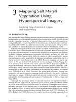
Network example 1: aggradation
Using NEA, it is possible to demonstrate how the connections that make up the network
are beneficial for the component and the entire ecosystem. Figure 5.2 presents a very sim-
ple example, presuming steady-state (inputϭ output) and first order donor determined
flows, which is often used in ecological modeling. Figure 5.2a shows the throughflow and
exergy storage (based on a retention time of five time units) in the two components with
no coupling, i.e., no network connections. Making a simple connection between the two
links them physically, and while it changes their individualistic behavior, it also alters the
overall system performance. In this case, the throughflow and exergy storage increase

because the part of the flow that previously exited the system is no used by the second
compartment, thereby increasing the total system throughflow, exergy stored, and average
path length. The advantages of integrated systems is also known from industrial ecology
in which waste from one industry can be used as raw material for another industry (see,
e.g., Gradel and Allenby, 1995; McDonough and Braungart, 2002; Jørgensen, 2006).
Network example 2: Cone Spring ecosystem
For the second example, we use the same Cone Spring ecosystem from the previous chap-
ter, which was used to demonstrate ascendency calculations (this will also help show the
88
A New Ecology: Systems Perspective
Box 5.2 Basic notation for network environ analysis
Flows: f
ij
ϭ within system flow directed from j to i, comprise a set of transactive
flows.
Boundary transfers: z
j
ϭ input to j, y
i
ϭ output from i.
Storages: x
j
represent n storage compartments (nodes).
Throughflow:
At steady-state:
Non-dimensional, intercompartmental flows are given by g
ij
ϭ f
ij
րT

j
Non-dimensional, intercompartmental utilities are given by d
ij
ϭ ( f
ij
Ϫf
ji
)րT
i
.
Non-dimensional, storage-specific, intercompartmental flows are given by
p
ij
ϭ c
ij
⌬t, where, for i j, c
ij
ϭ f
ij
րx
j
, and for iϭj, p
ii
ϭ 1ϩc
ii
⌬t, where c
ii
ϭϪT
i
րx

i
.
Non-dimensionless integral flow, storage, and utility intensity matrices, N, Q,
and U, respectively can be computed as the convergent power series:
(1)
The mth order terms, m ϭ 1,2,K, account for interflows over all pathways in the
system of lengths m.
NG G G G G (IG)
QP P P P P (IP)
U
0123 1
0123 1
ϭ ϩ ϩ ϩ ϩϩ ϩϭϪ
ϭ ϩ ϩ ϩ ϩϩ ϩϭϪ
ϭ
Ϫ
Ϫ
KK
KK
m
m
DDDDD D (ID)
012 3 1
ϩϩ ϩϩϩ ϩϭϪ
Ϫ
KK
m
TT T
ii i
(in) (out)

ϭ ϵ .
Tfy
iii
(out)
ϭϩ
Tzf
ii
(in)
ϭϩ
i
Else_SP-Jorgensen_ch005.qxd 4/12/2007 17:45 Page 88
similarities and differences between ascendency and environ analysis). Figure B4.1 shows
the flows in the system, but since the storage values are not given we limit ourselves here
to the flow and utility analyses. From the figure we obtain the following information (note,
flows are oriented from columns to rows):
A
00000
10111
01000
01100
00100
F
00000
8881 0 160
ϭϭ
⎡
⎣
⎢
⎢
⎢

⎢
⎢
⎢
⎤
⎦
⎥
⎥
⎥
⎥
⎥
⎥
00 200 167
0 5205 0 0 0
0 2309 75 0 0
0 0 370 0 0
11184
635
⎡
⎣
⎢
⎢
⎢
⎢
⎢
⎢
⎤
⎦
⎥
⎥
⎥

⎥
⎥
⎥
z ϭ 00
0
0
2303 3969 3530 1814 203
⎡
⎣
⎢
⎢
⎢
⎢
⎢
⎢
⎤
⎦
⎥
⎥
⎥
⎥
⎥
⎥
y ϭ[]
Chapter 5: Ecosystems have connectivity
89
A
50 exergy
units
B

50 exergy
units
10
10
10
10
5
10 5
15
10
10
7
5
2
13
10
a. No coupling between A and B. The throughflow is 20
and the exergy storage is 100 exergy units
b. A coupling from A to B. The throughflow is now 25
and the exergy storage is 125 exergy units.
A
50 exergy
units
B
75 exergy
units
c. A coupling from A to B and a coupling from B to A. The
throughflow is now 27 and the exergy storage is 135 exergy units
A
60 exergy

units
C
75 exergy
units
Figure 5.2 Two compartment system illustrating network aggradation as increased total system
throughflow and exergy storage relative to boundary inputs resulting from internal transactional
coupling. (a) no coupling. (b) one coupling. (c) cyclic coupling.
Else_SP-Jorgensen_ch005.qxd 4/12/2007 17:45 Page 89
Compartmental throughflow is the sum either entering OR exiting any compartment. At
steady-state these are equal, thus T
i
ϭ z
i
ϩ
j
f
ij
ϭ
j
f
ji
ϩ y
i
. Total system throughflow is
the sum of all compartmental throughflows: TSTϭ
j
T
i
, which here is 30,626 kcal/m
2

/y.
(Note, in ascendency analysis total system throughputϭ TSTϭ
nϩ2
i, jϭ1
T
ij
, which includes
both the input and output terms.) Continuing on with the NEA we present the non-
dimensional flow and utility matrices, G and D, respectively:
Running the analysis gives the integral flow matrix:
along with the following information: Finn Cycling Index is 0.0919, meaning about 9%
of flow is cycled flow, the ratio of direct to indirect flow is 0.9126, meaning that almost
half of all total system throughflow traveled along indirect paths (note, this is actually a
rare case exception when indirect flow contribution is not a majority), and the network
evenness measure (homogenization) is 2.0360, meaning that the values in integral flow
matrix, N, are twice as evenly distributed than the values in the direct flow matrix G—
which is evident just from eyeballing the two matrices. Another, important analysis pos-
sible with the flow data, but not displayed here is the calculation of the actual unit
environs, i.e., flow decompositions showing the amount of flow within the system “env-
iron” needed to generate one unit of input or output at each compartment. Unfortunately,
this particular example is one in which the powers of the utility matrix, D, do not guar-
antee convergence (since the maximum eigenvalue of D is greater than 1); and therefore,
N
1.000 0 0 0 0
0.958 1.207 0.374 0.186 0.545
0.434 0.547 1.169 0.084 0.ϭ 2247
0.199 0.251 0.092 1.039 0.113
0.031 0.039 0.014 0.161 1.018
⎡
⎣

⎢
⎢
⎢⎢
⎢
⎢
⎢
⎤
⎦
⎥
⎥
⎥
⎥
⎥
⎥
G
00000
0.794 0 0.308 0.084 0.451
0 0.453 0 0 0
0 0.201 0.014 0 0
0 0 0 0.155
ϭ
00
D
0 0.794 0 0 0
0.773 0 0.314 0.184 0.015
0 0.69
⎡
⎣
⎢
⎢

⎢
⎢
⎢
⎢
⎤
⎦
⎥
⎥
⎥
⎥
⎥
⎥
ϭ
Ϫ
ϪϪ
33 0 0.014 0
0 0.885 0.0315 0 0.155
0 0.451 0 1.00 0
Ϫ
Ϫ
Ϫ
⎡
⎣
⎢
⎢
⎢
⎢
⎢
⎢
⎤

⎦
⎥
⎥
⎥
⎥
⎥
⎥
90
A New Ecology: Systems Perspective
Else_SP-Jorgensen_ch005.qxd 4/12/2007 17:45 Page 90
we cannot present the synergism metrics. Although this is an area of ongoing research,
we can speculate about the ecological relationships in such cases by looking at the signs
of the utility matrices:
The direct utility matrix is zero-sum in that for every donor there is a receiver of the
flow. In ecological terms with think of a (ϩ, Ϫ) relationship as predation or exploita-
tion, but more generally it represents transfer from one compartment to another.
Matching compartments pair-wise across the main diagonal gives the relationship type
as shown in Table 5.2.
Notice, first that in the integral consideration that all compartments interact with
each other, not just directly—there are no zero elements in the matrix. Next, notice
that while two of the neutral direct relations became exploitation in one direction or
the other, two others became mutualistic relations. Furthermore, note that one direct
relations flipped when viewed in light of the system interactions—the relation
between compartments 2 and 5 was antagonistic in the direct sense, but mutualistic in
the holistic evaluation. The presence of each compartment benefits each other. Lastly,
note that overall the integral matrix has more positive signs than negative signs lead-
ing to a holistic emergence of network mutualism. See previous literature cited
(Patten, 1991, 1992; Fath and Patten, 1998; Fath, 2007) for other examples of utility
analysis calculations. Let us now turn to and end with a qualitative interpretation of
these network properties.

sgn(D)
0000
0
000
0+0
000
sgn(U)ϭ
Ϫ
ϩϪϪϩ
ϩϪ
ϩϪ
Ϫϩ
ϭ
ϩϪϩ
⎡
⎣
⎢
⎢
⎢
⎢
⎢
⎢
⎤
⎦
⎥
⎥
⎥
⎥
⎥
⎥

ϩϩϪ
ϩϩϪϪϩ
ϩϩϩϪϩ
ϩϩϪϩϪ
ϩϩϪϩϩ
⎡
⎣
⎢
⎢
⎢
⎢
⎢
⎢
⎤
⎦
⎥
⎥
⎥
⎥
⎥
⎥
Chapter 5: Ecosystems have connectivity
91
Table 5.2 Direct and integral relations for Cone Spring ecosystem
Direct Integral
(sd
21
, sd
12
)ϭ(ϩ, Ϫ) ; exploitation (sd

21
, sd
12
)ϭ(ϩ, Ϫ) ; exploitation
(su
31
, su
13
)ϭ(0, 0) ; neutralism (su
31
, su
13
)ϭ(ϩ, ϩ) ; mutualism
(su
41
, su
14
)ϭ(0, 0) ; neutralism (su
41
, su
14
)ϭ(ϩ, ϩ) ; mutualism
(su
51
, su
15
)ϭ(0, 0) ; neutralism (su
51
, su
15

)ϭ(ϩ, Ϫ) ; exploitation
(sd
32
, sd
23
)ϭ(ϩ, Ϫ) ; exploitation (sd
32
, sd
23
)ϭ(ϩ, Ϫ) ; exploitation
(sd
42
, sd
24
)ϭ(ϩ, Ϫ) ; exploitation (sd
42
, sd
24
)ϭ(ϩ, Ϫ) ; exploitation
(sd
52
, sd
25
)ϭ(Ϫ, ϩ) ; reverse exploitation (sd
52
, sd
25
)ϭ(ϩ, ϩ) ; mutualism
(sd
43

, sd
34
)ϭ(ϩ, Ϫ) ; exploitation (sd
43
, sd
34
)ϭ(Ϫ, Ϫ) ; competition
(su
53
, su
35
)ϭ(0, 0) ; neutralism (su
53
, su
35
)ϭ(Ϫ, ϩ) ; reverse exploitation
(sd
54
, sd
45
)ϭ(ϩ, Ϫ) ; exploitation (sd
54
, sd
45
)ϭ(ϩ, Ϫ) ; exploitation
Else_SP-Jorgensen_ch005.qxd 4/12/2007 17:45 Page 91
5.7 SUMMARY OF THE MAJOR INSIGHTS CARDINAL HYPOTHESES
(CH) FROM NETWORK ENVIRON ANALYSIS
CH-1: network pathway proliferation
After conservative substance enters a system through its boundary it is transacted—

conservatively transferred—between the living and non-living compartments within
the system, being variously transformed and reconfigured by work along the way. The
substance that enters as input to a particular compartment always while in the system
remains within the output environ of that, and only that, compartment. Thus, environs
as partition units within systems (Patten, 1978) defined by different inputs, become
entangled within and between the tangible components of the system (this is network
enfolding, another of the properties, discussed later). In accordance with second-law
requirements, a part (and eventually all) of this substance is continually dissipated back
to the environment by the entropy-generating processes that do work and make the sys-
tem function. At any point in time subsequent to initial introduction, remaining sub-
stance continues to be transported around the system, and as it does so it traces out
implicit pathways that extend in length by one unit at each transfer step. Pathway num-
bers increase exponentially with this increasing pathway length, with the result that the
interior of the system becomes a complex interconnected network in which all compo-
nents communicate, indirectly if not directly, with all or virtually all (depending on the
connectivity structure) the others. This pathway proliferation is thus one of the sources
of an essential holism, which environ theory impresses onto the interiors of systems.
And without the openness of semipermeable boundaries, pathways would neither begin
nor end, and the interior networks initiating output environs and terminating input
environs at boundary points of entry and exodus would never exist.
CH-2: network non-locality
As pathways extend the amount of substance carried along at any given step is less than
in the previous step due to dissipation. Therefore, pathways eventually end as they run
out of originally introduced material. The rate of decay can be expressed as an exponen-
tial function, just as is the rate of pathway proliferation. Dissipation and pathway exten-
sion and growth in numbers are in conflict, but early in the transactional sequence
following introduction the rate of the former exceeds that of the latter such that the total
substance transferred between compartment pairs over the aggregate of pathways of a
given length interconnecting them exceeds that of direct intercompartmental transfers. In
other words, indirect pathways (those of lengths Ͼ 2) deliver more substance from any

compartment to any other than a direct link between them. The influences carried by this
transferred substance follows the substance itself in its being associated with pathways of
particular lengths, and thus the conservative as well as non-conservative causes in the
system can be said to be non-local. Indirect effects are dominant in systems, and this is
especially true for complex systems, like ecosystems. The limit process that carries intro-
duced conservative substance throughout the system to ultimate dissipation ensures that
direct energy–matter links are quantitatively insignificant in comparison with the total.
These links, provided by direct interactions such as feeding, serve only to structure the
92
A New Ecology: Systems Perspective
Else_SP-Jorgensen_ch005.qxd 4/12/2007 17:45 Page 92
network; they make little contribution to intrasystem determination once this structuring
is established. Dominant indirect effects in nature—that is a very different proposition
from what we have in ecology at the present time. It is only a hypothesis, but robust in
the mathematics of steady-state environ analysis. And each extended pathway that col-
lectively provides its basis begins with openness at the boundary—either reception of
input followed by forward passage of material in output environs to ultimate dissipation,
or exhaustion from outputs preceded by the traceback of substance in input environs to
its boundary points of original introduction.
CH-3: network distributed control
Ecologists from the beginning of the subject have always been concerned with issues of
control—allogenic or autogenic—at physiological, population, community, and ecosys-
tem levels of organization. The subject permeates the discipline in many forms. There are
no obvious discrete controllers in ecosystems, though there are concepts like “key indus-
try organisms” and “keystone species” that are suggestive of such possibilities. In gen-
eral, in view of the non-locality property, control in ecosystems would have to be
considered as realized by dominantly indirect means. This is the postulate of distributed
control, and as with indirectness itself it is clear this has origins in boundary openness
(Patten and Auble, 1981; Fath, 2004; Schramski et al., 2006).
CH-4: network homogenization

Another consequence of non-locality is the tendency for intermediate sources and sinks
within systems to become blurred. That is, in the limit process that takes introduced
energy and matter to ultimate boundary dissipation, there is so much transactional
intercompartmental mixing around that causality tends to become evenly spread over
the interactive network. In the extreme, this means that all compartments in ecosystems
are about equally significant in generating and receiving influences to and from all the
others. Originating and terminating at the open boundaries of circumscribing systems,
the web of life based on local transactions of energy and matter tends to become quite
homogeneous in its unseen ultimate intercomponent relationships (Patten et al., 1990;
Fath and Patten, 1999).
CH-5: network internal amplification
It is sometimes observed in the environ mathematics of particular networks that sub-
stance introduced into one compartment at the boundary will appear more than once at
another compartment, despite boundary dissipation in the interim. This is due to recy-
cling, and it is easily seen how progressively diminishing fractions of a unit of introduced
substance can cumulatively produce a sum over time in a limit process that exceeds the
original amount. The second law cannot be defeated by this means, but energy cycling
(Patten, 1985) following from open boundaries can compensate it and make it appear at
least challenged in network organization. This is but one of numerous unexpected prop-
erties of networks contributed by cyclic interconnection and system openness.
Chapter 5: Ecosystems have connectivity
93
Else_SP-Jorgensen_ch005.qxd 4/12/2007 17:45 Page 93
CH-6: network unfolding
Ever since Raymond Lindeman (1942) pursued Charles Elton’s original food cycles, but
they came out unintendedly as sequential food chains instead, to which ecologists could
better relate, mainstream empirical ecology (e.g., food-web theory, biogeochemical
cycling) has had a difficult time returning to meaningful analysis of the concept of
cycling. The preoccupation with chains prompted Higashi and Burns (Higashi et al.,
1989) to develop a methodology for unfolding an arbitrary network into corresponding

isomorphic “macrochains.” Emanating from boundary points of input and arrayed pyra-
midally, these resemble the food pyramids of popular textbook depictions. Because the
networks are cyclic, however, the macrochains differ from normal acyclic food chains in
being indefinite in extent. Network unfolding refers to the indefinite proliferation of
substance-transfer levels in ecosystems. The terminology “transfer pathways” and “transfer
levels” is preferred to “food chains” and “trophic levels” because non-trophic as well as
trophic processes are involved in any realistic ecosystem. Examples of non-trophic
processes include import and export, anabolism and catabolism, egestion and excretion,
diffusion and convection, sequestering, immobilization, and so on. Whipple subsequently
modified the original unfolding methodology to discriminate the various trophic and
non-trophic processes involved (Whipple and Patten, 1993; Whipple, 1998). The transfer
levels so discriminated are non-discrete in containing contributions from most, if not all,
the compartments in a system, and also they continue to increase in accordance with con-
tinuation of the limit process that ultimately dissipates all the introduced substance from
the system. Exchange across open borders is at the heart of network unfolding.
CH-7: network synergism
The quantitative methodology of environ theory lends itself to development of certain
qualitative aspects of the environmental relation with organisms. Energy and matter are
objective quantities, but when cast as resources they engender subjective consequences
of having or not having them. A concept introduced in game theory (von Neumann and
Morgenstern, 1944, 1947) to describe the usefulness of outcomes or payoffs in games is
utility. Environ mathematics implements this concept to bridge the gap between objective
energy and matter and their subjective value as resources. Utility measures the relative
value of absolute quantities; it is subjective information extracted from and added onto
objective facts (Patten, 1991, 1992). A zero–sum game is one in which a winner gains
exactly what the loser loses. Each conservative transaction in ecosystems is zero-sum, but
it’s relative benefit to the gainer and loss to loser may be different. Network synergism
concerns how non-zero–sum interactions arise ultimately in conservative flow–storage
networks whose proximate transactional linkages are zero-sum (Fath and Patten, 1998).
Non-zero–sum interactions tend to be positive such that benefit/cost ratios, which equal

one in direct transactions, tend in absolute value to exceed one when non-local indirect
effects are taken into account. Such network synergism involves huge numbers of path-
ways (CH-1), dominant indirect effects (CH-2), and an indefinite transfer-level structure
that unfolds as a limit process (CH-6)—all features of utility generation that reflect
holistic organization in ecosystems, and the ecosphere. Once again—no open boundaries,
94
A New Ecology: Systems Perspective
Else_SP-Jorgensen_ch005.qxd 4/12/2007 17:45 Page 94
no interior networks, no transactional or relational (see immediately below) interactions,
and thus no non-zero-sum benefits to components. Life in networks is worth living, it can
be said, because the key property of openness as a necessary condition has made possi-
ble all subsequent properties derived from it.
CH-8: network mutualism
This property is a qualitative extension of the previous one (Patten, 1991, 1992). Every
compartment pair in a transactive network experiences positive (ϩ), negative (Ϫ), or
neutral relations derived from the transactions that directly and indirectly connect them.
Ordered pairs of these three signs are nine in number and each pair reflects a qualitative
interaction type. For example, the most common types of ecological interactions are
(ϩ, Ϫ) ϭ predation, (Ϫ, Ϫ) ϭ competition, (ϩ, ϩ) ϭ mutualism, and (0, 0) ϭ neutralism.
Since the signs of benefits and costs in network synergism are ϩ and Ϫ, respectively, the
shift to |benefit/cost| ratios Ͼ 1 in CH-7 carries with it a shift to positive interaction types.
This is network mutualism, and it indicates the benefits that automatically accrue to
living organisms by their being coupled into transactive networks. Network synergism
and mutualism together make nature a beneficial place conducive to life. This is quite
different from seeing life only as a Darwinian “struggle for existence”; it is true locally,
but not globally. There are built-in, openness-given properties of networks that, on
balance, operate to reduce the struggle.
CH-9: network aggradation
As stated above in network example 1, when energy or matter moves across a system
boundary, the system moves further from equilibrium and to that extent can be said to

aggrade thermodynamically, the opposite of dissipation (boundary exit) and degrada-
tion (energy destruction). Aggradation is negentropic, although entropy is still gener-
ated and boundary-dissipated by interior aggrading processes. Environ theory appears
to solve Schrödinger’s What-is-Life? riddle (1944) of how antientropic development
can proceed against the gradient of second-law degradation and dissipation. It shows
a necessary condition for aggradation to be one single interior transaction within the
interior system network—simple adjacent electromagnetic interaction! Given open-
ness and sustained boundary input and output, there would appear to be no upper
bound on this interior aggradation process. Thus, everything in nature that concerns
differentiation and diversification of living and non-living structures and processes,
and transactional interactions between these both within and across scales, can be seen
as incrementally contributing to network aggradation—movement away from equilib-
rium. Recalling the observation above that solar photons come in small quanta that
can only power processes at similarly small scales, and the fact that scales increase
bottom-up through interactive coupling, network aggradation would appear to pro-
vide, perhaps, an electromagnetic-coupling answer to Schödinger’s durable question,
“What is life?” Unbounded energy- and matter-based linkage following on boundary
openness would be an elegant basis indeed for life in its thermodynamic dimensions—
simple and ubiquitous.
Chapter 5: Ecosystems have connectivity
95
Else_SP-Jorgensen_ch005.qxd 4/12/2007 17:45 Page 95
CH-10: network boundary amplification
When a compartment within a system brings substance into the system from outside, the
importing compartment is favored in development over others that do not do this. The
reason is a technical property of both the throughflow- and storage-generating matrices
of environ analysis known as diagonal dominance. The throughflow case is easiest to
explain. Its generating matrix multiplies the system input vector to produce a through-
flow vector. Elements of the generating matrix represent the number of times substance
introduced at one compartment will appear in another. First introduction by boundary

input constitutes a first “hit” to the importing compartment. Non-importing compart-
ments do not receive such first hits. In matrix multiplication of the generating matrix and
input vector, importing compartments line up with their corresponding inputs such that
first hits are recorded in diagonal positions; that is, input z
i
to compartment i appears in
the iith position of the generating matrix. This alignment gives the diagonal dominance.
Off-diagonal elements represent contributions to i from the other interior compartments,
not across the boundary. These do not receive their first-hit from boundary input, but
from other interior compartments, and so are correspondingly smaller in numerical value.
Storage generation is similar. Elements of storage-generating matrices denote residence
times in each compartment of substance derived from other compartments. Diagonal
dominance in these generating matrices also associates longer residence times with
boundary vs. non-boundary inputs due to the first-hit phenomenon of the throughflow
model, and longer residence times result in greater standing stocks. Boundary amplifi-
cation may offer explanations for many phenomena in ecosystems—edge effects, zona-
tion, ecotones, trophic levels, etc. Take the latter as an example. The transfer levels of
network unfolding (CH-7) were seen to be non-discrete due to the mixing around of
energy matter in the complex network of indefinitely extending pathways. This negates
the mainstream Lindeman (1942) conception of discrete trophic levels. Boundary ampli-
fication restores discreteness, however, by giving another argument. Solar photons rep-
resent a resource initially outside the ecosystem boundary. Green plants bring them in
and thus plant life receives the first-hit advantage and ascends to planetary dominance as
a discrete trophic level, the primary producers. In a concentric, onion-like construction
of the ecosystem, the resultant living plant biomass represents an untapped resource lying
outside the possibilities for use (a functional boundary) until cellulose-digesting animals
evolve. When they do, the first-hit advantage establishes them as a second discrete
level—herbivores. These organisms initially lie outside the boundary of the next level
within, until flesh-eating animals can be developed to employ this resource. Their first-
hit advantage produces the third trophic level, carnivores. Omnivores evolve to utilize

herbivores and carnivores, and at this point the trophic-dynamic model begins to lose its
discreteness. All trophic levels produce dead organic residues, and the procaryotes and
eucaryotes were already in place over evolutionary time to utilize these; first-hit bound-
ary amplification establishes them as a discrete tropic category also—decomposers.
Boundary amplification is a relatively new property in environ theory. It has the poten-
tial to explain the emergence of discrete trophic levels within complex reticular networks,
and of course the more general property behind this is system openness.
96
A New Ecology: Systems Perspective
Else_SP-Jorgensen_ch005.qxd 4/12/2007 17:45 Page 96
CH-11: network enfolding
This property refers to the incorporation of indirect energy and matter flows and storages
into empirically observed and measured flows and storages. It is another property of
coupled systems elucidated by environ mathematics, and it potentially touches many
areas of ecology such as chemical stoichiometry, embodied energy (“emergy”), and
ecological indicators. Ecologists observe and measure, for example, the chemical
composition of organisms or bulk samples. For an entity to have a “composition” means
it is a composite—made up of materials brought to it from wherever its incoming network
reaches in the containing system—directly and indirectly. This has consequences for
even a seemingly straightforward concept like a “direct” flow where it turns out to be
“macroscopically direct” and must be distinguished from “microscopically direct.” To
illustrate, in Figure 5.2b the flow f
21
from compartment 1 to 2 is unambiguously direct.
Macroscopically, the link and the process responsible for it (like eating) are direct, and
microscopically so are the molecules (food) transferred because it is derived directly
from the boundary input z
1
. This latter directness is due to the fact that flow f
21

represents
the first transfer of boundary input from the compartment that received it to another; it is
uncontaminated by substance from other sources because, in this case, input z
2
cannot
reach compartment 1. The situation is different in Figure 5.3. The same flow f
21
in this
figure is still macroscopically adjacent to compartments 1 and 2 (i.e., “direct”), but now
it contains composited flow derived from all three inputs. These inputs, the throughflows
and storages (not shown) they generate, and also the other three adjacent flows are all
complexly enfolded into f
21
. The enfolding is mutual, and in this case it is universal
because all interior network elements are reachable from all the others. The entire system
of Figure 5.3 is thus (at steady-state) a composite of itself, which is the ultimate expres-
sion of holism. Moreover, this composition property, network enfolding, is true for com-
plex systems generally. If one can imagine empirically sampling this system, f
21
(and the
other interior flows as well) strike the senses as direct. However, they are not since they
contain indirect flows from the other sources a few to many times removed, and so are
better considered as “adjacent”, or perhaps just “observed.” In environ mathematics, this
Chapter 5: Ecosystems have connectivity
97
T
1
z
1
y

1
T
2
z
2
y
2
f
32
f
21
z
3
y
3
f
31
f
31

T
3
Figure 5.3 Three-compartment model illustrating network enfolding. Ecologically, the compart-
ment labeled T
1
can be taken as producers, T
2
as consumers, and T
3
as decomposers.

Else_SP-Jorgensen_ch005.qxd 4/12/2007 17:45 Page 97
embedding or entrainment of newly received inputs into the established flow-stream of
the system is reflected in infinite series. Let f
21
րT
1
ϭ g
21
define a throughflow-specific
dimensionless flow intensity. In effect g
21
is a probability, thus its powers form a convergent
infinite series: (1ϩg
21
ϩg
(2)
21
ϩLϩg
(m)
21
ϩL). The parenthesized superscripts denote
coefficients derived from matrix, not scalar, multiplication. This power series maps the
boundary input z
1
into the portion of throughflow at 2 contributed by this source:
T
21
ϭ(1ϩg
21
ϩg

(2)
21
ϩLϩg
(m)
21
ϩL) z
1
. The first term of the series brings the input into the
system: 1
и
z
1
. The second term represents the “direct” flow over the link of length 1: g
21
z
1
.
All other terms represent indirect flows associated with pathways of all lengths 2, 3, K,
m,Kas m;ϱ. The throughflow component T
21
accordingly contains a plethora of indirect
flows: (g
(2)
21
ϩLϩg
(m)
21
ϩL)z. This is one of three elements in the throughflow at compart-
ment 2: T
2

ϭT
21
ϩT
22
ϩT
23
. At compartment 1 the throughflow is similarly decomposable:
T
1
ϭT
11
ϩT
12
ϩT
13
, and at compartment 3: T
3
ϭT
31
ϩT
32
ϩT
33
. Each term in these sums
has a similar infinite series decomposition to that just given for T
21
. With this, one can now
appreciate there is more than that meets the eye in Figure 5.3. The focal flow f
21
in question

has a decomposition into enfolded elements as follows:
This is what an ecologist measuring f
21
would measure empirically and consider a
“direct” flow. One can see, however, that the entire system is embodied in this measure-
ment. This is network enfolding. It gives a strong message about the inherent holism one
can expect to be expressed in natural systems and, as stated above, its broad realization
is likely to influence many areas of ecology.
CH-12: network environ autonomy
One of the richer consequences of system openness is the extension of “selves” into the
broader surroundings that environ theory allows. Input and output environs extend
outward from their defining entities, and in a sense reflect and project, respectively, the
unique individuality of the latter in and into the world at large. Ownership of this “pro-
jection” is never released, however; the defining entities and their paired environs retain a
unity that cannot be disassembled, only decomposed, for example by mathematical analy-
sis. Moreover, as the entities themselves, particularly living ones, are unique, so also are
the environs they project. A careful reading of the consequences of organisms as open
systems having environments that uniquely attach to them is that not only are the
organisms autonomous, but so are their environs, although of necessity more diffusely
so. Estonian physiologist Jacob von Uexküll (1926) first put forward a view of the
organism–environment relationship that is not very far from the one environ theory
affords. Uexküll’s organisms had an incoming “world-as-sensed” and an outgoing “world-
of-action”, corresponding to input and output environs, respectively. He held that the
world-of-action wrapped around to the world-as-sensed via “function-circles” of the
fgTgTTT
ggg g z
m
21 21 1 21 11 12 13
21 11 11
(2)

11
()
1
()
1
ϭϭ ϩϩ
ϭϩϩϩϩϩ΄΂ ΃LLϩϩϩ ϩ ϩ ϩ ϩ
ϩϩ ϩ ϩ ϩ ϩ
΂΃
΂΃΅
1
1
12 12
(2)
12
()
2
13 13
(2)
13
()
3
gg g z
gg g z
m
m
LL
LL
98
A New Ecology: Systems Perspective

Else_SP-Jorgensen_ch005.qxd 4/12/2007 17:45 Page 98
organisms to produce an organism–environment complex that was a continuous whole, the
true functional unit of nature in principle, not the organism by itself. However, Uexküll
acknowledged the impossibility of tracing pathways of influence through the general envi-
ronment from outputs back to inputs, and to that extent the theoretical autonomy of his
organism–environment complexes was compromised. In environ theory, however, it is
possible to keep track of substances within system boundaries because the systems
involved are always models. In this case it can be demonstrated that each input and output
environ within a system has its own set of unique characteristics, and these have an
integrity and are maintained within the flow–storage stream of the model. The picture that
emerges is that environs—partition elements of larger networks—have integrity as consi-
tuted though diffuse units, and are indeed autonomous within the systems they occupy. All
measures of them that environ theory allows have never revealed two environs the same in
any of their characteristics. A given compartment in one environ will have, for a fixed unit
of boundary input or output, different flow, throughflow, storage, turnover and output char-
acteristics from the same compartment in other environs. Uexküll may have been more
correct than he realized when he wrapped his world-of-action around to his world-
as-sensed via his “functions circles” of the organism, and said that the entire existence of
the organism is imperilled should these function circles be interrupted.
CH-13: network holoevolution
The modern synthetic theory of biological evolution describes the evolutionary process in
terms of two fundamental phenomena—transgenerational descent, and modification of
descent over time. However, it only recognizes one kind of descent, genetic descent, and
one major modifying process, natural selection that is capable of steering genetic descent
non-randomly toward adaptive, fitness-maximizing configurations. Other modifying
processes, such as genetic drift and mutation, act at random. Thus, genetic fitness becomes
a matter of genes contributed by ancestral organisms to descendants via germ-line inheri-
tance. This “germ track” is separated from a corresponding body or “soma track” of non-
heritable, mortal phenotypes by the so-called “Weismann barrier” (1885). In the
post-Watson–Crick era of the second half of the 20th Century, this barrier came to mean

unidirectional DNA ; RNA ; protein coding. It ensures that “nothing that happens to
the soma can be communicated to the germ cells and their nuclei” (Mayr, 1982, p. 700).
This is genetic determinism—the doctrine that the structure and function of organisms are
exclusively determined by genes. The dogma has always been questioned, but it is now
under serious re-examination in systems biology (Klipp et al., 2005) as evidence mounts
showing the different ways environment controls gene expression. Environment is under-
played in conventional evolutionary theory, where it appears only as a non-specific agent
in natural selection. The environment of environ theory is two-sided, and both sides can
be seen to possess potentially heritable elements, enough to support the hypothesis that
environment and genomes both code for phenotypes, one from inside, the other from out-
side. The term envirotype has been coined to convey this idea Patten (in prep), and so
“holoevolution” (CH-13) postulates joint and balanced contributions to phenotypes, which
are mortal, from two evolutionary, potentially immortal, lines of inheritance. These are the
conventional genotype, engaged in bottom-up coding within the cell, and a corresponding
Chapter 5: Ecosystems have connectivity
99
Else_SP-Jorgensen_ch005.qxd 4/12/2007 17:45 Page 99
external envirotype, manifesting top-down coding from without. Both input and output
environs contribute to the heritable qualities of envirotypes, as outlined below:
•
Input-environ-based inheritance. We can begin with the cell, and then mentally extrapo-
late outward through higher levels of organization to the organism and beyond. Each
level, including that of the whole ecosystem, can be understood to have its own
mechanisms of receiving environmental information, generating responses to this, and
retaining (inheriting) through natural selection the ability to continue responses that
prove beneficial to survival. Consider a cell receiving an energy- or matter-based
signal from a near or distant source in its input environ. Biologist Bruce Lipton pres-
ents a scenario ( that effectively
breaches the Weismann barrier and allows transmission of environmental data directly
to the genome. Openness is at the heart of this process because the “cellular brain”, as

Lipton refers to it, is not located deep inside the cytoplasm or nucleus, but at the cell
boundary. It is the cell membrane, or plasmalemma, a crystalline bi-layer of phospho-
lipids and proteins that include a set of “integral membrane proteins” (IMPs) which
serve as receptors and effectors. Receptor proteins respond to incoming molecules, or
equally electromagnetic energy fields, by changing shape. This enables them to bond
with specific effector proteins (enzymes, cytoskeletal elements, or transporters of
electrons, protons, ions, or other chemical categories) that carry out behavior. If the
requisite effector proteins are not already present in the cytoplasm, the IMP percep-
tion units activate expression of appropriate genes in the nucleus to produce new ones.
New genes introduced into the DNA ; RNA ; protein sequence in the process
remain behind to be copied, enabling the response to be repeated if adaptive, or ulti-
mately fall obsolete and become consigned to the genomic set of inactive “junk”
genes. Correct activations lead to life-enhancing behaviors, incorrect ones to mal-
adaptation and death. Cellular adaptability thus becomes encoded in response to envi-
ronmental inputs into new genes that encode new proteins, enabling survival in
changing, but history-laden, environments. From the environ perspective, receptor
molecules respond to signals transmitted in input environs, and effector molecules
transmit the consequences to output environs. This initiates the second phase of envi-
ronmental inheritance.
•
Output-environ-based inheritance. When cells or other entities act on their environ-
ments the latter are changed as a result. This is “niche construction” Odling-Smee
et al. (2003). Its essence is that it alters the machinery of natural selection because
selection is, in the first instance, a manifestation of input environs. To the extent, how-
ever, that output environs generated by responses of their defining entities wrap
around and become elements in those entities’ input environs, the process becomes
heritable, and epiphenomena such as autoevolution (Lima de Faria, 1988) emerge as
distinct possibilities. Metazoan organization as “symbiogenic” aggregates of proto-
zoan antecedents (Margulis, 1981, 1991) is an example. This is based on wrap-around
feedback in which unicellular input- and output-environ overlaps are established in

multicellular organization and achieve integration and identity. Organized cell com-
munities possess self-similar IMP receptors responsive to the signal content of
100
A New Ecology: Systems Perspective
Else_SP-Jorgensen_ch005.qxd 4/12/2007 17:45 Page 100
hormones and other intercellular regulatory macromolecules. This requires that out-
put-environ elements become input-environ elements. Membrane proteins convert
adjacent environmental signals into cellular “awareness”, expressed as changes in pro-
tein configurations. The movements occasioned by these changes represent useful
kinetic energy (exergy) that does the work of achieving further departure from ther-
modynamic equilibrium, which multicellular organization represents compared to
unicells. This is the essence of all antientropic growth and development extending to
ecosystems and the ecosphere. Each level has mechanisms peculiar to it for
implementing environment-based inheritance and perpetuating all forms of life—
operational genotype–phenotype–envirotype complexes—through time. Organisms
and their cells below, and communities and ecosystems above, can be said to inherit
both their contained genes and attached environments from ancestral forms, and to the
extent that these environments manifest holism, the great panoply of life spread over
the globe at all levels of organization can be seen as evolving jointly, altogether, in the
ecosphere—“holoevolution.”
5.8 CONCLUSIONS
As evident throughout this chapter, ecosystems are networks of interacting biota and
abiota. Rigorous methodological tools such as input–output analysis and ecological
network analysis have been developed to deal with this complexity. As more and more
applications of systems and network analyses arise, it is important to remember the com-
mon methodological roots of the approaches. In fact, because of its basic assumption
about objects connected together as part of a larger system, which is used in several dis-
ciplines, the most promising application of network analysis may be as a platform for
integrated environmental assessment models to address sustainability issues of combined
human–natural systems.

Chapter 5: Ecosystems have connectivity
101
Else_SP-Jorgensen_ch005.qxd 4/12/2007 17:45 Page 101
This page intentionally left blank