A New Ecology - Systems Perspective - Chapter 6 doc

6
Ecosystems have complex dynamics
(growth and development)
Openness creates gradients
Gradients create possibilities
What you gain in precision,
you lose in plurality
(Thermodynamics and Ecological Modelling,
2000, S.E. Jørgensen (ed.))
6.1 VARIABILITY IN LIFE CONDITIONS
All known life on earth resides in the thin layer enveloping the globe known as the
ecosphere. This region extends from sea level to ϳ10km into the ocean depths and
approximately the same distance up into the atmosphere. It is so thin that if an apple were
enlarged to the size of the earth the ecosphere would be thinner than the peel. Yet a vast
and complex biodiversity has arisen in this region. Furthermore, the ecosphere acts as
integrator of abiotic factors on the planet accumulating in disproportionate quantities
particular elements favored by the biosphere (Table 6.1). In particular, note that carbon
is not readily abundant in the abiotic spheres yet is highly concentrated in the biosphere,
where nitrogen, silicon, and aluminum, while largely available, are mostly unincorporated.
However, even in this limited domain the conditions for living organisms may vary
enormously in time and space.
The climatic conditions:
(1) The temperature can vary from ϳϪ70 to ϳ55 centigrade.
(2) The wind speed can vary from 0km/h to several hundred km/h.
(3) The humidity may vary from almost 0–100 percent.
(4) The precipitation from a few millimeter in average per year to several meter per year,
which may or may not be seasonally aligned.
(5) Annual variation in day length according to latitude.
(6) Unpredictable extreme events such as tornadoes, hurricanes, earthquakes, tsunamis,
and volcanic eruptions.
103

Else_SP-Jorgensen_ch006.qxd 4/12/2007 17:59 Page 103
104
A New Ecology: Systems Perspective
The physical–chemical environmental conditions:
(1) Nutrient concentrations (C, P, N, S, Si, etc.)
(2) Salt concentrations (it is important both for terrestrial and aquatic ecosystems)
(3) Presence or absence of toxic compounds, whether they are natural or anthropogenic
in origin
(4) Rate of currents in aquatic ecosystems and hydraulic conductivity for soil
(5) Space requirements
The biological conditions:
(1) The concentrations of food for herbivore, carnivore, and omnivore organisms
(2) The density of predators
(3) The density of competitors for the resources (food, space, etc.)
(4) The concentrations of pollinators, symbiants, and mutualists
(5) The density of decomposers
The human impact on natural ecosystems today adds to this complexity.
The list of factors determining the life conditions is much longer—we have only men-
tioned the most important factors. In addition, the ecosystems have history or path
dependency (see Chapter 5), meaning that the initial conditions determine the possibili-
ties of development. If we modestly assume that 100 factors are defining the life condi-
tions and each of these 100 factors may be on 100 different levels, then 10
200
different
life conditions are possible, which can be compared with the number of elementary par-
ticle in the Universe 10
81
(see also Chapter 3). The confluence of path dependency and
an astronomical number of combinations affirms that the ecosphere could not experience
the entire range of possible states, otherwise known as non-ergodicity. Furthermore, its

irreversibility ensures that it cannot track back to other possible configurations. In addi-
tion to these combinations, the formation of ecological networks (see Chapter 5) means
that the number of indirect effects are magnitudes higher than the direct ones and they
are not negligible, on the contrary, they are often more significant than the direct ones,
as discussed in Chapter 5.
What is the result of this enormous variability in the natural life conditions? We have
found ϳ0.5ϫ10
7
species on earth and it is presumed that the number of species is
Table 6.1 Percent composition spheres for five most important elements
Lithosphere Atmosphere Hydrosphere Biosphere
Oxygen 62.5 Nitrogen 78.3 Hydrogen 65.4 Hydrogen 49.8
Silicon 21.22 Oxygen 21.0 Oxygen 33.0 Oxygen 24.9
Aluminum 6.47 Argon 0.93 Chloride 0.33 Carbon 24.9
Hydrogen 2.92 Carbon 0.03 Sodium 0.28 Nitrogen 0.27
Sodium 2.64 Neon 0.002 Magnesium 0.03 Calcium 0.073
Else_SP-Jorgensen_ch006.qxd 4/12/2007 17:59 Page 104
double or 10
7
. They have developed all types of mechanisms to live under the most var-
ied life conditions including ones at the margin of their physiological limits. They have
developed defense mechanisms. For example, some plants are toxic to avoid grazing,
others have thorns, etc. Animals have developed horns, camouflage pattern, well-developed
auditory sense, fast escaping rate, etc. They have furthermore developed integration
mechanisms; fitting into their local web of life, often complementing and creating their
environmental niche. The multiplicity of the life forms is inconceivable.
The number of species may be 10
7
, but living organisms are all different. An ecosystem
has normally from 10

15
to 10
20
individual organisms that are all different, which although
it is a lot, makes ecosystems middle number systems. This means that the number of
organisms is magnitudes less than the number of atoms in a room, but all the organisms,
opposite the atoms in the rooms, have individual characteristics. Whereas large number
systems such as the number of atoms in a room are amenable to statistical mechanics and
small number problems such as planetary systems to classical mechanics or individual
based modeling, middle number problems contain their own set of challenges. For one
thing this variation, within and among species, provides diversity through co-adaptation
and co-evolution, which is central both to Darwinian selection and network aggradation.
The competitive exclusion principle (Gause, 1934) claims that when two or more
species are competing about the same limited resource only the best one will survive. The
contrast between this principle and the number of species has for long time been a para-
dox. The explanation is rooted in the enormous variability in time and space of the con-
ditions and in the variability of a wide spectrum of species’ properties. A competition
model, where three or more resources are limiting gives a result very different from the
case where one or two resources are limiting. Due to significant fluctuations in the dif-
ferent resources it is prevented that one species would be dominant and the model
demonstrates that many species competing about the same spectrum of resources can
coexist. It is, therefore, not surprising that there exists many species in an environment
characterized by an enormous variation of abiotic and biotic factors.
To summarize the number of different life forms is enormous because there are a great
number of both challenges and opportunities. The complexity of ecosystem dynamics is
rooted in these two incomprehensible types of variability.
6.2 ECOSYSTEM DEVELOPMENT
Ecosystem development in general is a question of the energy, matter, and information
flows to and from the ecosystems. No transfer of energy is possible without matter and
information and no matter can be transferred without energy and information. The higher

the levels of information, the higher the utilization of matter and energy for further
development of ecosystems away from the thermodynamic equilibrium (see also
Chapters 2 and 4). These three factors are intimately intertwined in the fundamental
nature of complex adaptive systems such as ecosystems in contrast to physical systems,
that most often can be described completely by material and energy relations. Life is,
therefore, both a material and a non-material (informational) phenomenon. The self-
organization of life essentially proceeds by exchange of information.
Chapter 6: Ecosystems have complex dynamics (growth and development)
105
Else_SP-Jorgensen_ch006.qxd 4/12/2007 17:59 Page 105
E.P. Odum has described ecosystem development from the initial stage to the mature
stage as a result of continuous use of the self-design ability (E.P. Odum, 1969, 1971a);
see the significant differences between the two types of systems listed in Table 6.2 and
notice that the major differences are on the level of information. Table 6.2 show what we
often call E.P. Odum’s successional attributes, but also a few other concepts such as for
instance exergy and ecological networks have been introduced in the table.
106
A New Ecology: Systems Perspective
Table 6.2 Differences between initial stage and mature stage are indicated
Properties Early stages Late or mature stage
(A) Energetic
Production/respiration ϾϾ1 or ϽϽ1 Close to 1
Production/biomass High Low
Respiration/biomass High Low
Yield (relative) High Low
Specific entropy High Low
Entropy production
per unit of time Low High
Eco-exergy Low High
Information Low High

(B) Structure
Total biomass Small Large
Inorganic nutrients Extrabiotic Intrabiotic
Diversity, ecological Low High
Diversity, biological Low High
Patterns Poorly organized Well organized
Niche specialization Broad Narrow
Organism size Small Large
Life cycles Simple Complex
Mineral cycles Open Closed
Nutrient exchange rate Rapid Slow
Life span Short Long
Ecological network Simple Complex
(C) Selection and homeostasis
Internal symbiosis Undeveloped Developed
Stability (resistance to external
perturbations) Poor Good
Ecological buffer capacity Low High
Feedback control Poor Good
Growth form Rapid growth Feedback controlled
Growth types r-strategists K-strategists
Else_SP-Jorgensen_ch006.qxd 4/12/2007 17:59 Page 106
The information content increases in the course of ecological development because an
ecosystem integrates all the modifications that are imposed by the environment. Thus, it
is against the background of genetic information that systems develop which allow inter-
action of information with the environment. Herein lies the importance in the feedback
organism–environment, that means that an organism can only evolve in an evolving envi-
ronment, which in itself is modifying. The differences between the two stages include
entropy and eco-exergy.
The conservation laws of energy and matter set limits to the further development of

“pure” energy and matter, while information may be amplified (almost) without limit.
Limitation by matter is known from the concept of the limiting factor: growth continues
until the element which is the least abundant relatively to the needs by the organisms is
used up. Very often in developed ecosystems (for instance an old forest) the limiting ele-
ments are found entirely in organic compounds in the living organisms, while there is no
or very little inorganic forms left in the abiotic part of the ecosystem. The energy input
to ecosystems is determined by the solar radiation and, as we shall see later in this chap-
ter, many ecosystems capture ϳ75–80 percent of the solar radiation, which is their upper
physical limit. The eco-exergy, including genetic information content of, for example, a
human being, can be calculated by the use of Equations 6.2 and 6.3 (see also Box 6.3 and
Table 6.3). The results are ϳ40MJ/g.
A human body of ϳ80 kg will contain ϳ2 kg of proteins. If we presume that 0.01 ppt
of the protein at the most could form different enzymes that control the life processes and
therefore contain the information, 0.06 mg of protein will represent the information con-
tent. If we presume an average molecular weight of the amino acids making up the enzymes
of ϳ200, then the amount of amino acids would be 6ϫ10
Ϫ8
ϫ6.2ϫ10
23
ր200Ϸ2ϫ10
17
,
that would give an eco-exergy that is (10
Ϫ5
moles/g, Tϭ300K, 20 different amino acids):
It corresponds to 1.5ϫ 10
7
GJ/g. These are back of the envelope calculations and do not
represent what is expected to be the information content of organisms in the future; but
it seems possible to conclude that the development of the information content is very,

very far from reaching its limit, in contrast to the development of the material and energy
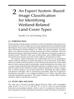
relations (see Figure 6.1).
Information has some properties that are very different from mass and energy.
(1) Information unlike matter and energy can disappear without trace. When a frog
dies the enormous information content of the living frog may still be there a
microseconds after the death in form of the right amino-acid sequences but the
information is useless and after a few days the organic polymer molecules have
decomposed.
(2) Information expressed for instance as eco-exergy, it means in energy units, is not
conserved. Property 1 is included in this property, but in addition it should be
stressed that living systems are able to multiply information by copying already
achieved successful information, which implies that the information survives and
ϭϫ ϫϫϫϫ ϭϫ
Ϫ
8.314 80,000 300 10 2 10 ln 20 1.2 10 GJ
517 12
Chapter 6: Ecosystems have complex dynamics (growth and development)
107
Else_SP-Jorgensen_ch006.qxd 4/12/2007 17:59 Page 107
108
A New Ecology: Systems Perspective
Table 6.3 -values for different organisms
Early organisms Plants Animals -values
Detritus 1.00
Virus 1.01
Minimal cell 5.8
bacteria 8.5
Archaea 13.8
Protists Algae 20
Yeast 17.8

Mesozoa, Placozoa 33
Protozoa, amoeba 39
Phasmida (stick insects) 43
Fungi, moulds 61
Nemertina 76
Cnidaria (corals, sea
anemones, jelly fish) 91
Rhodophyta 92
Gastroticha 97
Prolifera, sponges 98
Brachiopoda 109
Platyhelminthes (flatworms) 120
Nematoda (round worms) 133
Annelida (leeches) 133
Gnathostomulida 143
Mustard weed 143
Kinorhyncha 165
Seedless
vascular plants 158
Rotifera (wheel animals) 163
Entoprocta 164
Moss 174
Insecta (beetles, flies, bees,
wasps, bugs, ants) 167
Coleodiea (sea squirt) 191
Lipidoptera (buffer flies) 221
Crustaceans 232
Chordata 246
Rice 275
Gymnosperms

(inl. pinus) 314
(continued)
Else_SP-Jorgensen_ch006.qxd 4/12/2007 17:59 Page 108
thereby gives the organisms additional possibilities to survive. The information is
by autocatalysis (see Chapter 4) able to provide a pattern of biochemical processes
that ensure survival of the organisms under the prevailing conditions determined by
the physical–chemical conditions and the other organisms present in the ecosystem.
By the growth and reproduction of organisms the information embodied in the
genomes is copied. Growth and reproduction require input of food. If we calculate
Chapter 6: Ecosystems have complex dynamics (growth and development)
109
Mollusca, bivalvia,
gastropoda 310
Mosquito 322
Flowering plants 393
Fish 499
Amphibia 688
Reptilia 833
Aves (birds) 980
Mammalia 2127
Monkeys 2138
Anthropoid apes 2145
Homo sapiens 2173
Note: -values ϭ exergy content relatively to the exergy of detritus (Jørgensen et al., 2005).
Early organisms Plants Animals -values
Upper limit determined by limiting element and/or
energy captured.
Information
Present infor-
mation level

about 40MJ /g
Upper limit of information
in the order of 10^7 GJ /
g
Physical structure expressed
as energy /ha
Figure 6.1 While further development of physical structure is limited either by a limiting element
or by the amount of solar energy captured by the physical structure, the present most concentrated
amount of information, the human body, is very far from its limit.
Table 6.3 (Continued)
Else_SP-Jorgensen_ch006.qxd 4/12/2007 17:59 Page 109
the eco-exergy of the food as just the about mentioned average of 18.7kJ/g, the gain
in eco-exergy may be more; but if we include in the energy content of the food the
exergy content of the food, when it was a living organism or maybe even what the
energy cost of the entire evolution has been, the gain in eco-exergy will be less than
the eco-exergy of the food consumed. Another possibility is to apply emergy instead
of energy. Emergy is defined later in this chapter (Box 6.2). The emergy of the food
would be calculated as the amount of solar energy it takes to provide the food, which
would require multiplication by a weighting factor ϾϾ 1.
(3) The disappearance and the copying of information, that are characteristic processes
for living systems, are irreversible processes. A made copy cannot be taken back and
the death is an irreversible process. Although information can be expressed as eco-
exergy in energy units it is not possible to recover chemical energy from information
on the molecular level as know from the genomes. It would require a Maxwell’s
Demon that could sort out the molecules and it would, therefore, violate the second
law of thermodynamics. There are, however, challenges to the second law (e.g., Capek
and Sheehan, 2005) and this process of copying information could be considered one
of them. Note that since the big bang enormous amounts of matter have been con-
verted to energy (Eϭmc
2

) in a form that makes it impossible directly to convert the
energy again to mass. Similarly, the conversion of energy to information that is char-
acteristic for many biological processes cannot be reversed directly in most cases. The
transformation matter ;energy;molecular information, which can be copied at low
cost is possible on earth, but these transformation processes are irreversible.
(4) Exchange of information is communication and it is this that brings about the self-
organization of life. Life is an immense communication process that happens in
several hierarchical levels (Box 2.2). Exchange of information is possible with a very
tiny consumption of energy, while storage of information requires that the informa-
tion is linked to material, for instance are the genetic information stored in the
genomes and is transferred to the amino-acid sequence.
A major design principle observed in natural systems is the feedback of energy from
storages to stimulate the inflow pathways as a reward from receiver storage to the
inflow source (H.T. Odum, 1971b). See also the “centripetality” in Chapter 4. By this
feature the flow values developed reinforce the processes that are doing useful work.
Feedback allows the circuit to learn. A wider use of the self-organization ability of
ecosystems in environmental or rather ecological management has been proposed by
H.T. Odum (1983, 1988).
E.P. Odum’s idea of using attributes to describe the development and the conditions of
an ecosystem has been modified and developed further during the past 15 years. Here we
assess ecosystem development using ecological orientors to indicate that the develop-
ment is not necessarily following in all details E.P. Odum’s attributes because ecosystems
are ontically open (Chapter 3). In addition, it is also rare that we can obtain data to
demonstrate the validity of the attributes in complete detail. This recent development is
presented in the next section.
110
A New Ecology: Systems Perspective
Else_SP-Jorgensen_ch006.qxd 4/12/2007 17:59 Page 110
The concept of ecological indicators has been introduced ϳ15–20 years ago. These
metrics indicate the ecosystem condition or the ecosystem health, and are widely used to

understand ecosystem dynamics in an environmental management context. E.P. Odum’s
attributes could be used as ecological indicators; but also specific indicator species that show
with their presence or absence that the ecosystem is either healthy or not, are used. Specific
contaminants that indicate a specific disease are used as indicators. Finally, it should be men-
tioned that indicators such as biodiversity or thermodynamic variables are used to indicate a
holistic image of the ecosystems’ condition; further details see Chapter 10. The relationship
between biodiversity and stability was previously widely discussed (e.g., May, 1973), who
showed that there is not a simple relationship between biodiversity and stability of ecosys-
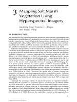
tems. Tilman and his coworkers (Tilman and Downing, 1994) have shown that temperate
grassland plots with more species have a greater resistance or buffer capacity to the effect of
drought (a smaller change in biomass between a drought year and a normal year). However,
there is a limit—each additional plant contributed less (see Figure 6.2). Previously, it has
been shown that for models there is a strong correlation between eco-exergy (the definition;
see Chapter 2) and the sum of many different buffer capacities. Many experiments (Tilman
and Downing, 1994) have also shown that higher biodiversity increases the biomass and
therefore the eco-exergy. There is in other words a relationship between biodiversity and eco-
exergy and resistance or buffer capacity.
Box 6.1 gives the definitions for ecological orientors and ecological indicators. In eco-
logical modeling, goal functions are used to develop structurally dynamic models. Also
the definition of this third concept is included in the box.
Chapter 6: Ecosystems have complex dynamics (growth and development)
111
Number of s
p
ecies
0 10 20 25
Drough resistance
-0.5
-1.0
-1.5

Figure 6.2 Results of the Tilman and Downing (1994) grassland experiments. The higher the
number of species the higher the drought buffer capacity, although the gain per additional plant
species decreasing with the number of species.
Else_SP-Jorgensen_ch006.qxd 4/12/2007 17:59 Page 111
It has been possible theoretically to divide most of E.P. Odum’s attributes into three
groups, defining three different growth and development forms for ecosystems
(Jørgensen et al., 2000):
I. Biomass growth that is an attribute and also explains why P/B and R/B decreases
with the development and the nutrients go from extrabiotic to intrabiotic pools.
II. Network growth that corresponds directly to increased complexity of the ecological
network, more complex life and mineral cycles, a slower nutrient exchange rate and
a more narrow niche specialization. It also implies a longer retention time in the
system for energy and matter.
III. Information growth that explains the higher diversity, larger animals, longer life span,
more symbiosis and feed back control and a shift from r-strategists to K-strategists.
IV. In addition, we may of course also have boundary growth—increased input, as we can
observe for instance for energy during the spring. It is this initial boundary flow that
is a prerequisite for maintaining ecosystems as open far-from-equilibrium systems.
6.3 ORIENTORS AND SUCCESSION THEORIES
The orientor approach that was briefly introduced above, describes ideal-typical trajec-
tories of ecological properties on an integrated ecosystem level. Therefore, it follows the
traditions of various concepts in ecological theory, which are related to environmental
dynamics. A significant example is succession theory, describing “directional processes
of colonization and extinction of species in a given site” (Dierssen, 2000). Although
there are big intersections, these conceptual relationships have not become sufficiently
obvious in the past, due to several reasons, which are mainly based on methodological
problems and critical opinions which have been discussed eagerly after the release of
112
A New Ecology: Systems Perspective
Box 6.1 Definitions of orientors, indicators, and goal functions

Ecological orientors: Ecosystem variables that describe the range of directions in
which ecosystems have a propensity to develop. The word orientors is used to indicate
that we cannot give complete details about the development, only the direction.
Ecological indicators: These indicate the present ecosystem condition or health. Many
different indicators have been used such as specific species, specific contaminants,
indices giving the composition of groups of organisms (for instance an algae index),
E.P. Odum’s attributes and holistic indicators included biodiversity and thermodynamic
variables such as entropy or exergy.
Ecological goal functions: Ecosystems do not have defined goals, but their propensity
to move in a specific direction indicated by ecological orientors, can be described in
ecological models by goal functions. Clearly, in a model, the description of the
development of the state variables of the model has to be rigorously indicated, which
implies that goals are made explicit. The concept should only be used in ecological
modeling context.
Else_SP-Jorgensen_ch006.qxd 4/12/2007 17:59 Page 112
Odum’s paper on the strategy of ecosystem development (1969). Which were the
reasons for these controversies?
Traditional succession theory is basically oriented toward vegetation dynamics. The
pioneers of succession research, Clements (1916) and Gleason (1917) were focusing
mainly on vegetation. Consequently, also the succession definitions of Whittacker (1953),
Egler (1954), Grime (1979), or Picket et al. (1987) are related to plant communities, while
heterotrophic organisms often are neglected (e.g., Horn, 1974; Connell and Slayter, 1977).
Therefore, also the conclusions of the respective investigations often have to be reduced
to the development of vegetation components of ecosystems, while the orientor approach
refers to the whole ensemble of organismic and abiotic subsystems and their interrelations.
These conceptual distinctions for sure are preferable sources for misunderstandings.
A sufficient number of long-term data sets are not available. Therefore, as some authors
state throughout the discussions of Odum’s “strategy” paper (1969), the theoretical pre-
dictions of succession theory seem to be “based on untested assumptions or analogies”
(e.g., Drury and Nisbet, 1973; Horn, 1974; Connell and Slayter, 1977), while there is only

small empirical evidence. This situation becomes even more problematic if ecosystem data
are necessary to test the theoretical hypotheses. Consequently, we will also in future have
to cope with this lack of data, but we can use more and more empirical investigations,
referring to the orientor principle, which have been reported in the literature (e.g., Marques
et al., 2003; Müller et al., i.p.). We can hope for additional results from ecosystem analy-
ses and Long Term Ecological Research Programs. Meanwhile validated models can be
used as productive tools for the analysis of ecosystem dynamics.
The conceptual starting points differ enormously. Referring to the general objections
against the maturity concept, Connell and Slayter (1977) funnel their heavy criticism
about Odum’s 24 ecosystem features into the questions of whether mature communities
really are “internally controlled” and if “steady states really are maintained by internal
feedback mechanisms”. Having doubts in these facts, they state that, therefore, no char-
acteristics can be deduced from this idea. Today, there is no doubt about the existence of
self-organizing processes in all ecosystems (e.g., Jørgensen, 2002). Of course there are
exterior constraints, but within the specific degrees of freedom, in fact the internal regu-
lation processes are responsible for the development of ecosystems. Hence, the basic
argument against the maturity concept has lost weight throughout the years.
Comparing successional dynamics, often different spatial and temporal scales are mixed.
This point is related to the typical time scales of ecological investigations. They are most
often carried out in a time span 2–4 years. Of course it is very difficult to draw conclu-
sions over centuries from these short-term data sets. Also using paleo-ecological methods
give rise to broad uncertainties, and when spatial differences are used to represent the
steps of temporal developments, the questions of the site comparability introduces prob-
lems which might reduce the evidence of the findings enormously. Furthermore, there is
the general problem of scale. If we transfer short-term results to long-term processes,
then we cannot be sure to use the right algorithms and to take into account the correct,
scale conform constraints and processes (O’Neill et al., 1986). And, looking at the spatial
scale, the shifting mosaic hypothesis (Remmert, 1991) has shown that there will be huge
Chapter 6: Ecosystems have complex dynamics (growth and development)
113

Else_SP-Jorgensen_ch006.qxd 4/12/2007 17:59 Page 113
differences if different spatial extents are taken into account, and that local instabilities
can be leading to regional steady-state situations. What we can see is that there are many
empirical traps we can fall into. Maybe the connection of empirical research and ecologi-
cal modeling can be helpful as a “mechanism of self-control” in this context.
Due to the “ontic openness” of ecosystems, predictability in general is rather small but in
many cases exceptions can be found. The resulting dilemma of a system’s inherent uncer-
tainty can be regarded as a consequence of the internal complexity of ecosystems, the
non-linear character of the internal interactions and the often-unforeseeable dynamics of
environmental constraints. Early on, succession researchers found the fundamentals of
this argument, which are broadly accepted today. The non-deterministic potential of eco-
logical developments has already been introduced in Tansley’s (1953) polyclimax theory,
which is based on the multiple environmental influences that function as constraints for
the development of an ecosystem. Simberloff (1982) formulates that “the deterministic
path of succession, in the strictest Clementsian mono-climax formulation, is as much an
abstraction as the Newtonian particle trajectory” and Whittaker (1972) states, “the vege-
tation on the earth’s surface is in incessant flux”. Stochastic elements, complex interac-
tions, and spatial heterogeneities take such important influences that the idea of Odum
(1983) that “community changes…are predictable”, must be considered in relative terms
today, if detailed prognoses (e.g., on the species level) are desired. But this does not mean
that general developmental tendencies can be avoided, i.e. this fact does not contradict the
general sequence of growth forms as formulated in this volume. Quite the opposite: this
concept realizes the fact that not all ecosystem features are optimized throughout the
whole sequence, a fact that has been pointed out by Drury and Nisbet (1973) and others.
Disturbances are causes for separating theoretical prognoses from practical observations.
One example for these non-deterministic events is disturbance, which plays a major role
in ecosystem development (e.g., Drury and Nisbet, 1973; Sousa, 1984). Odum (1983) has
postulated that succession “culminates in the establishment of as stable an ecosystem as
its biologically possible on the site in question” and he notes that mature communities are
able to buffer the physical environment to a greater extent than the young community. In

his view stability and homoeostasis can be seen as the result (he even speaks about a
purpose) of ecological succession from the evolutionary standpoint. But in between, the
guiding paradigm has changed: today Holling’s adaptive cycling model (1986) has
become a prominent concept, and destruction is acknowledged as an important compo-
nent of the continuous adaptation of ecosystems to changing environmental constraints.
This idea also includes the feature of brittleness in mature states, which can support the
role of disturbance as a setting of new starting points for an oriented development.
Terminology has inhibited the acceptance of acceptable ideas. The utilization of terms
like “strategy”, “purpose”, or “goal” has led to the feeling that holistic attitudes toward
ecological successions in general are loaded with a broad teleological bias. Critical col-
leagues argued that some of these theories are imputing ecosystems to be “intentionally”
following a certain target or target state. This is not correct: the series of states is a con-
sequence of internal feedback processes that are influenced by exterior constraints and
impulses. The finally achieved attractor state thus is a result, not a cause.
114
A New Ecology: Systems Perspective
Else_SP-Jorgensen_ch006.qxd 4/12/2007 17:59 Page 114
Summarizing, many of the objections against the initial theoretical concepts of ecosys-
tem development and especially against the stability paradigm have proven to be correct,
and they have been modified in between. Analogies are not used anymore, and the number
of empirical tests is increasing. On the other hand, the theory of self-organization has clar-
ified many critical objections. Thus, a consensus can be reached if cooperation between
theory and empiricism is enhanced in the future.
6.4 THE MAXIMUM POWER PRINCIPLE
Lotka (1925, 1956) formulated the maximum power principle. He suggested that systems
prevail that develop designs that maximize the flow of useful (for maintenance and
growth) energy, and Odum used this principle to explain much about the structure and
processes of ecosystems (Odum and Pinkerton, 1955). Boltzmann (1905) said that the
struggle for existence is a struggle for free energy available for work, which is a defini-
tion very close to the maximum exergy principle introduced in the next section. Similarly,

Schrödinger (1946) pointed out that organization is maintained by extracting order from
the environment. These two last principles may be interpreted as the systems that are able
to gain the most free energy under the given conditions, i.e. to move most away from the
thermodynamic equilibrium will prevail. Such systems will gain most biogeochemical
energy available for doing work and therefore have most energy stored to use for main-
tenance and buffer against perturbations.
H.T. Odum (1983) defines the maximum power principle as a maximization of useful
power. It is applied on the ecosystem level by summing up all the contributions to the
total power that are useful. It means, that non-useful power is not included in the sum-
mation. Usually the maximum power is found as the sum of all flows expressed often in
energy terms for instance kJ/24h.
Brown et al. (1993) and Brown (1995) has restated the maximum power principle in
more biological terms. According to the restatement it is the transformation of energy
into work (consistent with the term useful power) that determines success and fitness.
Many ecologists have incorrectly assumed that natural selection tends to increase effi-
ciency. If this were true, then endothermy could never have evolved. Endothermic birds
and mammals are extremely inefficient compared with reptiles and amphibians. They
expend energy at high rates in order to maintain a high, constant body temperature,
which, however, gives high levels of activities independent of environmental temperature
(Turner, 1970). Brown (1995) defines fitness as reproductive power, dW/dt, the rate at
which energy can be transformed into work to produce offspring. This interpretation of
the maximum power principle is even more consistent with the maximum exergy princi-
ple that is introduced in the next section, than with Lotka’s and Odum’s original idea.
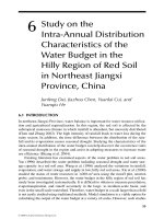
In the book Maximum Power: The Ideas and Applications of H.T. Odum, Hall (1995)
has presented a clear interpretation of the maximum power principle, as it has been
applied in ecology by H.T. Odum. The principle claims that power or output of useful
work is maximized, not the efficiency and not the rate, but the tradeoff between a high
rate and high efficiency yielding most useful energy or useful work. It is illustrated in
Figure 6.3.
Chapter 6: Ecosystems have complex dynamics (growth and development)

115
Else_SP-Jorgensen_ch006.qxd 4/12/2007 17:59 Page 115
Hall is using an interesting semi-natural experiment to illustrate the application of the
principle in ecology. Streams were stocked with different levels of predatory cutthroat
trout. When predator density was low, there was considerable invertebrate food per pred-
ator, and the fish used relatively little maintenance energy searching for food per unit of
food obtained. With a higher fish-stocking rate, food became less available per fish, and
each fish had to use more energy searching for it. Maximum production occurred at inter-
mediate fish-stocking rates, which means intermediate rates at which the fish utilized
their food.
Hall (1995) mentions another example. Deciduous forests in moist and wet climates
tend to have a leaf area index (LAI) of ϳ6 m
2
/m
2
. Such an index is predicted from the
maximum power hypothesis applied to the net energy derived from photosynthesis.
Higher LAI values produce more photosynthate, but do so less efficiently because of the
metabolic demand of the additional leaf. Lower leaf area indices are more efficient per
leaf, but draw less power than the observed intermediate values of roughly 6.
The same concept applies for regular fossil fuel power generation. The upper limit of
efficiency for any thermal machine such as a turbine is determined by the Carnot effi-
ciency. A steam turbine could run at 80 percent efficiency, but it would need to operate
at a nearly infinitely slow rate. Obviously, we are not interested in a machine that gener-
ates electricity or revenues infinitely slowly, no matter how efficiently. Actual operating
efficiencies for modern steam powered generator are, therefore, closer to 40 percent,
roughly half the Carnot efficiency.
These examples show that the maximum power principle is embedded in the irre-
versibility of the world. The highest process efficiency can be obtained by endo-reversible
conditions, meaning that all irreversibilities are located in the coupling of the system to its

surroundings, there are no internal irreversibilities. Such systems will, however, operate
116
A New Ecology: Systems Perspective
Rate
Efficiency
Power output
Low rate, high
efficiency
High rate, low
efficiency
Figure 6.3 The maximum power principle claims that the development of an ecosystem is a
tradeoff (a compromise) between the rate and the efficiency, i.e. the maximum power output per
unit of time.
Else_SP-Jorgensen_ch006.qxd 4/12/2007 17:59 Page 116
too slowly. Power is zero for any endo-reversible system. If we want to increase the process
rate, it will imply that we also increase the irreversibility and thereby decrease the effi-
ciency. The maximum power is the compromise between endo-reversible processes and
very fast completely irreversible processes.
The concept of emergy (embodied energy) was introduced by H.T. Odum (1983) and
attempts to account for the energy required in formation of organisms in different trophic
levels. The idea is to correct energy flows for their quality. Energies of different types are
converted into equivalents of the same type by multiplying by the energy transformation
ratio. For example fish, zooplankton, and phytoplankton can be compared by multiplying
their actual energy content by their solar energy transformation ratios. The more trans-
formation steps there are between two kinds of energy, the greater the quality and the
greater the solar energy required to produce a unit of energy (J) of that type. When one
calculates the energy of one type, that generates a flow of another, this is sometimes
referred to as the embodied energy of that type. Figure 6.4 presents the concept of
embodied energy in a hierarchical chain of energy transformation. One of the properties
of high quality energies is their flexibility (which requires information). Whereas low

quality products tend to be special, requiring special uses, the higher quality part of a web
is of a form that can be fed back as an amplifier to many different web components.
Chapter 6: Ecosystems have complex dynamics (growth and development)
117
SUN
1000 100 10 1
kJ / m
2
h
Solar Equivalents kJ / m
2
h
Energy Transformation Ratios =
Embodied Energy Equivalents.
kJ / m
2
h
1000
SUN
1000 1000
1 10 100 1000
SUN
1000
Figure 6.4 Energy flow, solar equivalents, and energy transformation ratiosϭembodied energy
equivalents in a food chain (Jørgensen, 2002).
Else_SP-Jorgensen_ch006.qxd 4/12/2007 17:59 Page 117
A good down to earth example of what emergy is, might be the following: in 1 year
one human can survive on 500 fish each of the size of 500g, that may have consumed
80,000 frogs with the size of 20g. The frogs may have eaten 18ϫ 10
6

insects of the size
of 1 g. The insects have got their food from 200,000 kg dry matter of plants. As the pho-
tosynthetic net production has an efficiency of 1 percent, the plants have required an
input of ϳ3.7ϫ 10
9
J, presuming an energy content of plant dry matter of 18.7 kJ/g. To
keep one human alive costs, therefore 3.7ϫ 10
9
J, although the energy stock value of a
human being is only in the order 3.7ϫ10
5
J or 10,000 times less. The transformity is,
therefore, 10,000.
H.T. Odum has revised the maximum power principle by replacing power with
emergy–power (empower), meaning that all the contributions to power are multiplied by a
solar equivalent factor that is named transformity to obtain solar equivalent joules (sej)
(see Box 6.2). The difference between embodied energy flows and power, see Equation 6.1,
simply seems to be a conversion to solar energy equivalents of the free energy.
118
A New Ecology: Systems Perspective
Box 6.2 Emergy
“Emergy is the available energy of one kind previously used up directly and indirectly
to make a service or product. Its unit is the emjoule [(ej)]” and its physical dimensions
are those of energy (Odum, 1996). In general, since solar energy is the basis for all
the energy flows in the biosphere, we use solar emergy (measured in sej, solar
emjoules), the solar energy equivalents required (directly or indirectly) to make a
product.
The total emergy flowing through a system over some unit time, referenced to its
boundary source, is its empower, with units [sej/(time)] (Odum, 1988). If a system, and
in particular an ecosystem, can be considered in a relatively steady state, the empower

(or emergy flow) can be seen as nature’s “labor” required for maintaining that state.
The emergy approach starts from Lotka’s maximum power principle (1922, 1956) and
corrects the function, which is maximized, since not all the energy types have the same
ability of doing actual work. Thus power (flow of energy) is substituted by empower
(flow of emergy), that is “in the competition among self-organizing processes, network
designs that maximize empower will prevail” (Odum, 1996).
Transformity is the ratio of emergy necessary for a process to occur to the exergy
output of the process. It is an intensive function and it is dimensionless, even though
sej/J is used as unit.
Emergy can be written as a function of transformity and exergy as follows (i identi-
fies the inputs):
While transformity can be written as

kkk
Em Exϭ ͞
Em Ex
i
i
i
ϭ 
∑
Else_SP-Jorgensen_ch006.qxd 4/12/2007 17:59 Page 118
Chapter 6: Ecosystems have complex dynamics (growth and development)
119
even though it is often calculated as
By definition the transformity of sunlight is equal to 1 and this assumption avoids the
circularity of these expressions. All the transformities (except that of solar energy)
are, therefore, greater than 1.
Transformities are always measured relative to a planetary solar emergy baseline and
care should be taken to ensure that the transformities used in any particular analysis

are all expressed relative to the same baseline (Hall, 1995). However, all the past
baselines can be easily related through multiplication by an appropriate factor and
the results of an emergy analysis do not change by shifting the baseline (Odum,
1996).
Emergy and transformity are not state functions, i.e. they strongly depend on the
process that is used to obtain a certain item. There are transformities that are
calculated from global biosphere data (i.e. rain, wind, geothermal heat) and others
that, being the result of more complex and variable processes have high vari-
ability: for example, electricity can be generated by many processes (using wood,
water, coal, gas, tide, solar radiation, etc.) each with a different transformity
(Odum, 1996).
In general transformity can be seen as a measure of “quality”: while emergy, follow-
ing “memorization” laws, can in general remain constant or grow along transforma-
tion chains, since as energy decreases, transformities increase. On the other hand,
when comparing homologous products, the lower the transformity, the higher the effi-
ciency in transforming solar emergy into a final product.
Emergy is a donor-referenced concept and a measure of convergence of energies,
space and time, both from global environmental work and human services into a
product. It is sometimes referred to as “energy memory” (Scienceman, 1987) and
its logic (of “memorization” rather than “conservation”) is different from other
energy-based analyses as shown by the emergy “algebra”. The rules of emergy
analysis are:
•
All source emergy to a process is assigned to the processes’ output.
•
By-products from a process have the total emergy assigned to each pathway.
•
When a pathway splits, the emergy is assigned to each ‘leg’ of the split based on
its percentage of the total energy flow on the pathway.
•

Emergy cannot be counted twice within a system: (a) emergy in feedbacks cannot
be double counted; (b) by-products, when reunited, cannot be added to equal a sum
greater than the source emergy from which they were derived.
For in depth discussion of this issue and the differences between energy and emergy
analysis see Odum (1996).

k
k
k
Em
Ex
ϭ
ր
ր
time
time
Else_SP-Jorgensen_ch006.qxd 4/12/2007 17:59 Page 119
Embodied energy is, as seen from these definitions, determined by the biogeochemi-
cal energy flow into an ecosystem component, measured in solar energy equivalents. The
stored emergy, Em, per unit of area or volume to be distinguished from the emergy flows
can be found from:
(6.1)
where 
i
is the quality factor which is the conversion to solar equivalents, as illustrated
in Figure 6.4, and c
i
is the concentration expressed per unit of area or volume.
The calculations reduce the difference between stored emergy (= embodied energy)
and stored exergy (see next section), to the energy quality factor. The quality factor for

exergy accounts for the information embodied in the various components in the system
(detailed information is given in the next section), while the quality factor for emergy
accounts for the solar energy cost to form the various components. Emergy calculates
thereby how much solar energy (which is our ultimate energy resource) it has taken to
obtain 1 unit of biomass of various organisms. Both concepts attempt to account for the
quality of the energy. Emergy by looking into the energy flows in the ecological network
to express the energy costs in solar equivalents. Exergy by considering the amount of bio-
mass and information that has accumulated in that organism. One is measure of the path
that was taken to get to a certain configuration, the other a measure of the organisms in
that configuration.
6.5 EXERGY, ASCENDENCY, GRADIENTS, AND ECOSYSTEM
DEVELOPMENT
Second law dissipation acts to tear down structure and eliminate gradients, but ecosys-
tems have the ability to move away from thermodynamic equilibrium in spite of the
second law dissipation due to an inflow of energy from solar radiation. Even a simple
physical system as a Bernard cell is using an inflow of energy to move away from ther-
modynamic equilibrium. A Bernard cell consists of two plates, that are horizontally
placed in water a few centimeter from each other. The lower plate has higher temperature
than the upper plate. Consequently, energy is flowing from the lower to the upper plate.
When the temperature difference is low the motion of the molecules is random. When the
temperature exceeds a critical value the water molecules are organized in a convection
pattern, series of rolls or hexagons. The energy flow increases due to the convection. The
greater the flow of energy the steeper the temperature gradient (remember that work
capacityϭ entropy times temperature gradient) and the more complex the resulting struc-
ture. Therefore, greater exergy flow moves the system further away from thermodynamic
equilibrium—higher temperature gradient and more ordered structure containing
information corresponding to the order. The origin of ordered structures is, therefore,
openness and a flow of energy (see Chapter 2). Openness and a flow of energy are both
necessary conditions (because it will always cost energy to maintain an ordered structure)
and sufficient (as illustrated with the Bernard cell). Morowitz (1968, 1992) has shown

that an inflow of energy always will create one cycle of matter, which is an ordered
Em c
ii
i
n
ϭ
ϭ

1
∑
120
A New Ecology: Systems Perspective
Else_SP-Jorgensen_ch006.qxd 4/12/2007 17:59 Page 120
structure. Openness and a flow of energy is, however, not sufficient condition for ecosys-
tems (see Chapter 2), as additional conditions are required to ensure that the ordered
structure is an ecosystem.
Biological systems, especially, have many possibilities for moving away from
thermodynamic equilibrium, and it is important to know along which pathways among
the possible ones a system will develop. This leads to the following hypothesis
(Jørgensen and Mejer, 1977, 1979; Jørgensen, 1982, 2001, 2002; Jørgensen et al., 2000):
if a system receives an input of exergy, then it will utilize this exergy to perform work.
The work performed is first applied to maintain the system (far) away from thermo-
dynamic equilibrium whereby exergy is lost by transformation into heat at the tem-
perature of the environment. If more exergy is available, then the system is moved
further away from thermodynamic equilibrium, reflected in growth of gradients. If
there is offered more than one pathway to depart from equilibrium, then the one yield-
ing the highest eco-exergy storage (denoted Ex) will tend to be selected. Or expressed
differently: among the many ways for ecosystems to move away from thermodynamic
equilibrium, the one maximizing dEx/dt under the prevailing conditions will have a
propensity to be selected.

Rutger de Wit (2005) has expressed preference for a formulation where the flow of
exergy is replaced by a flow of free energy, which of course is fully acceptable and makes
the formulation closer to classic thermodynamics. However, eco-exergy storage can
hardly be replaced by free energy because it is a free-energy difference between the sys-
tem and the same system at thermodynamic equilibrium. The reference state is therefore
different from ecosystem to ecosystems, which is considered in the definition of eco-
exergy. In addition, free energy is not a state function far from thermodynamic equili-
brium—just consider the immediate loss of eco-exergy when an organism dies. Before
the death the organism has high eco-exergy because it can utilize the enormous informa-
tion that is embodied in the organism, but at death the organism loses immediately the
ability to use this information that becomes, therefore, worthless. Moreover, the infor-
mation part of the eco-exergy cannot be utilized directly as work; see the properties of
information presented in Section 6.2.
Just as it is not possible to prove the three laws of thermodynamics by deductive
methods, so can the above hypothesis only be “proved” inductively. A number of con-
crete cases which contribute generally to the support of the hypothesis will be pre-
sented below and in Chapters 8 and 9. Models are often used in this context to test the
hypothesis. The exergy can be approximated by use of the calculation methods in
Box 6.3. Strictly speaking exergy is a measure of the useful work which can be per-
formed. Conceptually, this obviously includes the energetic content of the material,
i.e. biomass, but also the state of organization of the material. One way to measure the
organization is the information content of the material, which could be the complex-
ity at the genetic or ecosystem levels. Currently, the organizational aspect of exergy is
expressed as Kullbach’s measure of information based on the genetic complexity of
the organism:
(6.2)
Ex B RT Kϭ
Chapter 6: Ecosystems have complex dynamics (growth and development)
121
Else_SP-Jorgensen_ch006.qxd 4/12/2007 17:59 Page 121

where B is the biomass, R the gas constant, T the Kelvin temperature, and K Kullbach’s
measure of information (further details see Box 6.3). The exergy of the organism is found
on basis of the information that the organism carries:
(6.3)
where Ex
i
is the exergy of the ith species, 
i
a weighting factor that considers the infor-
mation the ith species is carrying in c
i
(Table 6.2). Jørgensen et al. (2005) show how
the -values have been found for different organisms. A high uncertainty is, however,
associated with the assessment of the -values, which implies that the exergy calcula-
tions have a corresponding high uncertainty. In addition, the exergy is calculated based
on models that are simplifications of the real ecosystems. The calculated exergy
should, therefore, only be used relatively and considered an index and not a real
absolute exergy value.
Ex c
iii
ϭ 
122
A New Ecology: Systems Perspective
Box 6.3 Calculation of eco-exergy
It is possible to distinguish between the exergy of information and of biomass
(Svirezhev, 1998). p
i
defined as c
i
/B, where

is the total amount of matter in the system, is introduced as new variable in Equation 2.8:
As the biomass is the same for the system and the reference system, BϷB
o
exergy
becomes a product of the total biomass B (multiplied by RT ) and Kullback measure:
where p
i
and p
i,o
are probability distributions, a posteriori and a priori to an observa-
tion of the molecular detail of the system. It means that K expresses the amount of
information that is gained as a result of the observations. If we observe a system that
consists of two connected chambers, then we expect the molecules to be equally
distributed in the two chambers, i.e. p
1
ϭ p
2
ϭ 1/2. If we, on the other hand, observe
that all the molecules are in one chamber, we get p
1
ϭ 1 and p
2
ϭ 0.
Specific exergy is exergy relatively to the biomass and for the ith component:
Sp. ex.
i
ϭ Ex
i
/c
i

. It implies that the total specific exergy per unit of area or per unit of
volume of the ecosystem is equal to RTK.
Kp
p
p
i
i
io
i
n
ϭ
ϭ
ln
,
1
∑
Ex B RT p
p
p
B
B
B
i
i
io
i
n
o
ϭϩ
ϭ

ln ln
,
1
∑
Bc
i
i
n
ϭ
ϭ1
∑
Else_SP-Jorgensen_ch006.qxd 4/12/2007 17:59 Page 122
Consistency of the exergy-storage hypothesis, as we may call it, with other theories
(goal functions, orientors; see Sections 6.2 and 6.3) describing ecosystem development
will be demonstrated as a pattern in a later section of this chapter. It should, however, in
this context be mentioned that exergy storage in the above-mentioned main hypothesis
can be replaced by maximum power. Exergy focuses on the storage of biomass (energy)
and information, while power considers the energy flows resulting from the storages.
Chapter 6: Ecosystems have complex dynamics (growth and development)
123
For the components of the ecosystem, 1 (covers detritus), 2, 3, 4.K N, the proba-
bility, p
1,o
, consists at least of the probability of producing the organic matter (detri-
tus), i.e. p
1,o
, and the probability, p
i,a
, to find the correct composition of the enzymes
determining the biochemical processes in the organisms. Living organisms use 20 dif-

ferent amino acids and each gene determines on average a sequence of ϳ700 amino
acids (Li and Grauer, 1991). p
i,a
, can be found from the number of permutations
among which the characteristic amino-acid sequence for the considered organism has
been selected.
The total exergy can be found by summing up the contributions originating from
all components. The contribution by inorganic matter can be neglected as the contri-
butions by detritus and even to a higher extent from the biological components are
much higher due to an extremely low probability of these components in the reference
system. Roughly, the more complex (developed) the organism is the more enzymes
with the right amino-acid sequence are needed to control the life processes, and there-
fore the lower is the probability p
i,a
, The probability p
i,a
, for various organisms has
been found on basis of our knowledge about the genes that determine the amino-acid
sequence. As the concentrations are multiplied by RT and ln ( p
i
/p
i,o
), denoted 
i
; a
table with the -values for different organisms have been prepared (see Table 6.3). The
contribution by detritus, dead organic matter, is in average 18.7kJ/g times the con-
centration (in g/unit of volume). The exergy can now be calculated by the following
equation:
The -values are found from Table 6.3 and the concentration from modeling or obser-

vations. By multiplication by 18.7, we get the exergy in kilojoules.
Notice that
while
Ex c
ii
i
n
info
1
( 1) (asdetritusequivalent)ϭϪ
ϭ

∑
Ex c
i
i
n
bio
1
(asdetritusequivalent)ϭ
ϭ
∑
Exergy total (asdetritusequivalent)
1
ϭ
ϭ

ii
i
n

c
∑
Else_SP-Jorgensen_ch006.qxd 4/12/2007 17:59 Page 123
Ascendency (Box 4.1) is a complex measure of the information and flows embodied
the ecological network. The definition is given in Chapter 4. At the crux of ascendency
lies the action of autocatalysis (Chapter 4). One of the chief attributes of autocatalysis is
what Ulanowicz (1997) calls “centripetality” or the tendency to draw increasing amounts
of matter and energy into the orbit of the participating members (Chapter 4). This ten-
dency inflates ascendency both in the quantitative sense of increasing total system activ-
ity and qualitatively by accentuating the connections in the loop above and beyond
pathways connecting non-participating members. At the same time, increasing storage of
exergy is a particular manifestation of the centripetal tendency, and the dissipation of
external exergy gradients to feed system autocatalysis describes centripetality in an
almost tautological fashion.
In retrospect, the elucidation of the connections among ascendency, eco-exergy, and
aggradation (Ulanowicz et al., 2006) has been effected by stages that are typical of theory-
driven research. First, it was noted in phenomenological fashion how quantitative obser-
vations of the properties were strongly correlated; the correlation coefficient, r
2
, was
found for a number of models to be 0.99 (Jørgensen, 1995). Thereafter, formal definitions
were used to forge theoretical ties among the separate measures. Finally, the perspective
offered by these new theoretical connections facilitated a verbal description of the com-
mon unitary agency that gave rise to the independent trends that had been formalized as
separate principles. Eco-exergy and ascendency represent two sides of the same coin or
two different angles in the description of ecosystem development. A simple physical phe-
nomenon as light requires both a description as waves and as particle to be fully under-
stood. It is, therefore, understandable that ecosystem developments that are much more
complicated than light require multiple description. Exergy covers the storage, maximum
power the flows, and ascendency the ecological network and all three concepts contribute

to the overall aggradation, moving away from thermodynamic equilibrium. All three con-
cepts have well-structured roots in the theoretical soil. Their shortcomings are, however,
that calculations of exergy, maximum power, and ascendency always will be incomplete
due to the enormous complexity of ecosystems (see Section 6.1).
Ecosystems can also be understood as a (high) number of interacting gradients, which
are formed by self-organizing processes (Mueller and Leupelt, 1998). Gradient mainte-
nance costs exergy that is transformed by decomposition processes to heat at the tem-
perature of the environment, i.e. the exergy is lost. The gradients can be classified in
various ways, but we could also distinguish three types of gradients corresponding to the
three growth forms (see Section 6.2): gradients due to organisms in the ecosystems (trees
are good illustrations), gradients due to formation of a more complex network (for
instance the spatial distribution of more or fewer niches), and gradients due to
information (the level of information could be used directly as illustration). The first-
mentioned class of gradients requires the most exergy for maintenance, while informa-
tion gradients require very little or no exergy for maintenance. Gradients summation is
captured in the exergy measure since work capacity is an extensive variable times a gra-
dient (see Chapter 2).
Exergy storage is the simplest of the three concepts to calculate; but clearly the assess-
ment of the -values has some shortcomings. The latest list is more differentiated than
124
A New Ecology: Systems Perspective
Else_SP-Jorgensen_ch006.qxd 4/12/2007 17:59 Page 124
the previous ones (Jørgensen et al., 1995; Fonseca et al., 2000) and is based on the latest
results of the entire genome analyses for 11 species plus a series of complexity measures
for a number of species, families, orders, or classes. The list will most probably be
improved as genetics gains more information about the genomes and proteomes of more
species. The total information of an ecosystem should furthermore include the informa-
tion of the network. All ecological models that are used as basis for the exergy calcula-
tions are much simpler than the real network and the information contained in the
network of the model become negligible compared to the exergy in the compartments. A

calculation method to assess the information of the real ecological network is needed to
account for the contribution to the total ecosystem exergy.
Power is very difficult to assess because the ecological observations are mostly based
on concentrations and not on flows, which implies that it is hardly possible to validate the
flow values resulting from ecological models. In addition, the number of flows in the real
ecological network is magnitudes higher than the few flows that can be included in our
primitive calculations.
Calculations of ascendency have the same shortcomings as calculations of power.
The three concepts may all have a solid theoretical basis but their applications in prac-
tice still have definite weaknesses that are rooted in the complexity of real ecosystems.
Based on an integration of the three concepts, we are able to expand on the earlier hypo-
thesis based on exergy alone and let it comprise acendency and power in addition to exergy.
6.6 SUPPORT FOR THE PRESENTED HYPOTHESES
Below are presented a few case studies from Jørgensen (2002) and Jørgensen et al. (2000)
supporting the presented exergy storage hypothesis, but maximum power or ascendency
could also have been applied as discussed in Section 6.5. More examples can be found in
these references and in Chapter 8.
1. Size of genomes
In general, biological evolution has been toward organisms with an increasing number of
genes and diversity of cell types (Futuyima, 1986). If a direct correspondence between
free energy and genome size is assumed, then this can reasonably be taken to reflect
increasing exergy storage accompanying the increased information content and process-
ing of “higher” organisms.
2. Le Chatelier’s principle
The exergy storage hypothesis might be taken as a generalized version of “Le Chatelier’s
Principle.” Biomass synthesis can be expressed as a chemical reaction:
(6.4)
According to Le Chatelier’s Principle, if energy is put into a reaction system at equili-
brium, then the system will shift its equilibrium composition in a way to counteract the
energy nutrients molecules with morefree energy (exergy) and orgϩϭ aanization

dissipated energyϩ
Chapter 6: Ecosystems have complex dynamics (growth and development)
125
Else_SP-Jorgensen_ch006.qxd 4/12/2007 17:59 Page 125
change. This means that more molecules with more free energy and organization will be
formed. If more pathways are offered, then those giving the most relief from the distur-
bance (displacement from equilibrium) by using the most energy, and forming the most
molecules with the most free energy, will be the ones followed in restoring equilibrium.
3. The sequence of organic matter oxidation
The sequence of biological organic matter oxidation (e.g., Schlesinger, 1997) takes place
in the following order: by oxygen, by nitrate, by manganese dioxide, by iron (III), by sul-
phate, and by carbon dioxide. This means that oxygen, if present, will always out com-
pete nitrate which will out compete manganese dioxide, and so on. The amount of exergy
stored as a result of an oxidation process is measured by the available kJ/mole of elec-
trons which determines the number of adenosine triphosphate molecules (ATPs) formed.
ATP represents an exergy storage of 42kJ/mole. Usable energy as exergy in ATPs
decreases in the same sequence as indicated above. This is as expected if the exergy stor-
age hypothesis were valid (Table 6.4). If more oxidizing agents are offered to a system,
the one giving the highest storage of free energy will be selected.
In Table 6.3, the first (aerobic) reaction will always out compete the others because it
gives the highest yield of stored exergy. The last (anaerobic) reaction produces methane;
this is a less complete oxidation than the first because methane has a greater exergy con-
tent than water.
4. Formation of organic matter in the primeval atmosphere
Numerous experiments have been performed to imitate the formation of organic matter
in the primeval atmosphere on earth 4 billion years ago (Morowitz, 1968). Energy from
various sources were sent through a gas mixture of carbon dioxide, ammonia, and
methane. There are obviously many pathways to utilize the energy sent through simple
gas mixtures, but mainly those forming compounds with rather large free energies (amino
acids and RNA-like molecules with high exergy storage, decomposed when the

compounds are oxidized again to carbon dioxide, ammonia and methane) will form an
appreciable part of the mixture (according to Morowitz, 1968).
126
A New Ecology: Systems Perspective
Table 6.4 Yields of kJ and ATP’s per mole of electrons, corresponding to 0.25 moles of CH
2
O
oxidized (carbohydrates)
1
Reaction kJ/mole e
Ϫ
ATP’s/mole e
Ϫ
CH
2
Oϩ O
2
ϭ CO
2
ϩ H
2
O 125 2.98
CH
2
Oϩ 0.8 NO
3
–ϩ 0.8 H
+
ϭ CO
2

ϩ 0.4 N
2
ϩ 1.4 H
2
119 2.83
CH
2
Oϩ 2 MnO
2
ϩ H
ϩ
ϭ CO
2
ϩ 2 Mn
2ϩ
ϩ 3 H
2
O 85 2.02
CH
2
Oϩ 4 FeOOHϩ 8 H
ϩ
ϭ CO
2
ϩ 7 H
2
Oϩ Fe
2ϩ
27 0.64
CH

2
Oϩ 0.5 SO
4
2Ϫ
ϩ 0.5 H
ϩ
ϭ CO
2
ϩ 0.5 HS
Ϫ
ϩ H
2
O 26 0.62
CH
2
Oϩ 0.5 CO
2
ϭ CO
2
ϩ 0.5 CH
4
23 0.55
1
The released energy is available to build ATP for various oxidation processes of organic matter at pH 7.0
and 25° C.
Else_SP-Jorgensen_ch006.qxd 4/12/2007 17:59 Page 126
5. Photosynthesis
There are three biochemical pathways for photosynthesis: (1) the C3 or Calvin–Benson
cycle, (2) the C4 pathway, and (3) the Crassulacean acid metabolism (CAM) pathway.
The latter is least efficient in terms of the amount of plant biomass formed per unit of

energy received. Plants using the CAM pathway are, however, able to survive in harsh,
arid environments that would be inhospitable to C3 and C4 plants. CAM photosynthesis
will generally switch to C3 as soon as sufficient water becomes available (Shugart, 1998).
The CAM pathways yield the highest biomass production, reflecting exergy storage,
under arid conditions, while the other two give highest net production (exergy storage)
under other conditions. While it is true that a gram of plant biomass produced by the three
pathways has different free energies in each case, in a general way improved biomass pro-
duction by any of the pathways can be taken to be in a direction that is consistent, under
the conditions, with the exergy storage hypothesis.
6. Leaf size
Givnish and Vermelj (1976) observed that leaves optimize their size (thus mass) for the con-
ditions. This may be interpreted as meaning that they maximize their free-energy content.
The larger the leaves the higher their respiration and evapotranspiration, but the more solar
radiation they can capture. Deciduous forests in moist climates have a LAI of ϳ6 m
2
/m
2
(see
also Section 2.4). Such an index can be predicted from the hypothesis of highest possible
leaf size, resulting from the tradeoff between having leaves of a given size versus maintain-
ing leaves of a given size (Givnish and Vermelj, 1976). Size of leaves in a given environ-
ment depends on the solar radiation and humidity regime, and while, for example, sun and
shade leaves on the same plant would not have equal exergy contents, in a general way leaf
size and LAI relationships are consistent with the hypothesis of maximum exergy storage.
7. Biomass packing
The general relationship between animal body weight, W, and population density, D, is
Dϭ A/W, where A is a constant (Peters, 1983). Highest packing of biomass depends only
on the aggregate mass, not the size of individual organisms. This means that it is biomass
rather than population size that is maximized in an ecosystem, as density (number per
unit area) is inversely proportional to the weight of the organisms. Of course the rela-

tionship is complex. A given mass of mice would not contain the same exergy or number
of individuals as an equivalent weight of elephants. Also, genome differences (Example 1)
and other factors would figure in. Later we will discuss exergy dissipation as an alterna-
tive objective function proposed for thermodynamic systems. If this were maximized
rather than storage, then biomass packing would follow the relationship Dϭ A/W
0.65–0.75
(Peters, 1983). As this is not the case, biomass packing and the free energy associated
with this lend general support for the exergy storage hypothesis.
8. Cycling
If a resource (for instance, a limiting nutrient for plant growth) is abundant, then it will
typically recycle faster. This is a little strange because recycling is not needed when a
Chapter 6: Ecosystems have complex dynamics (growth and development)
127
Else_SP-Jorgensen_ch006.qxd 4/12/2007 17:59 Page 127