A New Ecology - Systems Perspective - Chapter 8 docx

8
Ecosystem principles have broad
explanatory power in ecology
THE BEST ANSWER RAISES MOST QUESTIONS
8.1 INTRODUCTION
The criticism that ecology as a whole lacks universal laws and predictive theory is fre-
quent, and there are authors who even argue that theoretical ecology concerned for
instance with fitness and natural selection is not scientific (Murray, 2001).
Scientific observations on natural phenomena usually give origin to possible explana-
tions and, furthermore, provide tentative generalizations that may lead to broad-scale
comprehension of the available information. Generalizations may be descriptive and
inductive, deriving from observations carried out on observable characteristics, or
become much more eager, constituting the base of deductive theories. In ecology, we
must recognize that there are basically no universal laws (maybe such laws cannot even
exist in the same sense as those in physics). In fact, most explanations in ecology are
inductive generalizations, without any deductive theory behind them, and as a conse-
quence we may find a large number of non-universal tentative generalizations.
As explained earlier in the book, regarding features such as immense number prob-
lem, growth and decay, and network interrelations, ecology is more complex than
physics, and it will, therefore, be much more difficult to develop an applicable, predic-
tive ecological theory. Testing explanatory hypotheses by verification instead of by falsi-
fication is perhaps the easiest way. But many ecologists probably feel inwards the need
for a more general and integrative theory that may help in explaining their observations
and experimental results.
In the last 20 or 30 years several new ideas, approaches, and hypotheses appeared in
the field of systems ecology, which when analyzed more deeply appear to form a pat-
tern of theories able to explain the dynamics of ecosystems (Jørgensen, 1997, 2002).
And in fact, due to the complexity involved, we probably need a number of different
complementary approaches to explain ecosystem structure and function (Jørgensen,
1994a; Fath et al., 2001). Such ecosystem theories were only used in a limited way in
ecological modeling, namely in the development of non-stationary models, able to take

into account the adaptation of biological components (Jørgensen, 1986, 1992b, 1994b,
1997; Jørgensen and de Bernardi, 1997, 1998). It has been argued that to improve sub-
stantially the predictive power of ecological models it will probably be necessary to
apply theoretical approaches much more widely (Jørgensen and Marques, 2001).
167
Else_SP-Jorgensen_ch008.qxd 3/29/2007 09:59 Page 167
168
A New Ecology: Systems Perspective
Nevertheless, the question remains: is it possible to develop a theoretical framework
able to explain the numerous observations, rules, and correlations dispersed in the eco-
logical literature during the last few decades?
Although we may have no sound answer to this question, it has been argued (Jørgensen
and Marques, 2001) that it should at least be possible to propose a promising direction for
ecological thinking. The idea in this chapter is to check the compliance of ecosystem prin-
ciples to a number of ecological rules or laws, and to see if other proposed non-universal
explanations provided by different authors about different ecological problems can be
further enlightened according to the same ecological principles.
8.2 DO ECOLOGICAL PRINCIPLES ENCOMPASS OTHER PROPOSED
ECOLOGICAL THEORIES?: EVOLUTIONARY THEORY
One of the most important, if not the most important, theories in biology is the theory of
evolution; so we begin by outlining this theory, with examples and with intent later to
show a similarity with it to the ecosystem theories proposed earlier in the book. In bio-
logy, evolution is the process by which natural populations of organisms acquire and pass
on novel characteristics from generation to generation (Darwin and Wallace, 1858;
Darwin, 1859), and the theory of evolution by natural selection became decisively esta-
blished within the scientific community. In the 1930s, work by a number of scientists
combined Darwinian natural selection with the re-discovered theory of heredity (proposed
by Gregor Mendel) to create the modern evolutionary synthesis. In the modern synthesis,
“evolution” means a change in the frequency of an allele within a gene pool from one
generation to the next. This change may be caused by a number of different mechanisms:

natural selection, genetic drift, or changes in population structure (gene flow).
(a) Natural selection is survival and reproduction as a result of the environment.
Differential mortality consists of the survival rate of individuals to their reproductive
age. Differential fertility is the total genetic contribution to the next generation. The
central role of natural selection in evolutionary theory has given rise to a strong con-
nection between that field and the study of ecology.
Natural selection can be subdivided into two categories:
•
Ecological selection occurs when organisms that survive and reproduce increase
the frequency of their genes in the gene pool over those that do not survive.
•
Sexual selection occurs when organisms that are more attractive to the opposite sex
because of their features reproduce more and thus increase the frequency of those
features in the gene pool.
Natural selection also operates on mutations in several different ways:
•
Purifying or background selection eliminates deleterious mutations from a
population.
•
Positive selection increases the frequency of a beneficial mutation.
Else_SP-Jorgensen_ch008.qxd 3/29/2007 09:59 Page 168
•
Balancing selection maintains variation within a population through a number of
mechanisms, including:
••
Over-dominance or heterozygote advantage, where the heterozygote is more fit
than either of the homozygous forms (exemplified by human sickle cell anemia
conferring resistance to malaria).
••
Frequency-dependent selection, where the rare variants have a higher fitness.

•
Stabilizing selection favors average characteristics in a population, thus reducing
gene variation but retaining the mean.
•
Directional selection favors one extreme of a characteristic; results in a shift in the
mean in the direction of the extreme.
•
Disruptive selection favors both extremes, and results in a bimodal distribution of
gene frequency. The mean may or may not shift.
(b) Genetic drift describes changes in allele frequency from one generation to the next
due to sampling variance. The frequency of an allele in the offspring generation will
vary according to a probability distribution of the frequency of the allele in the par-
ent generation.
Many aspects of genetic drift depend on the size of the population (generally abbreviated
as N ). This is especially important in small mating populations, where chance fluctua-
tions from generation to generation can be large. Such fluctuations in allele frequency
between successive generations may result in some alleles disappearing from the popu-
lation. Two separate populations that begin with the same allele frequency might, there-
fore, “drift” by random fluctuation into two divergent populations with different allele
sets (e.g. alleles that are present in one have been lost in the other).
The relative importance of natural selection and genetic drift in determining the fate
of new mutations also depends on the population size and the strength of selection: when
N
·
s (population size times strength of selection) is small, genetic drift predominates.
When N
·
s is large, selection predominates. Thus, natural selection is ‘more efficient’ in
large populations, or equivalently, genetic drift is stronger in small populations. Finally,
the time for an allele to become fixed in the population by genetic drift (i.e. for all indi-

viduals in the population to carry that allele) depends on population size, with smaller
populations requiring a shorter time to fixation.
The theory underlying the modern synthesis has three major aspects:
(1) The common descent of all organisms from a single ancestor.
(2) The manifestation of novel traits in a lineage.
(3) The mechanisms that cause some traits to persist while others perish.
Essentially, the modern synthesis (or neo-Darwinism) introduced the connection
between two important discoveries: the evolutionary units (genes) with its mechanism
(selection). It also represents a unification of several branches of biology that previously
had little in common, particularly genetics, cytology, systematics, botany, and paleontology.
Chapter 8: Ecosystem principles have broad explanatory power in ecology
169
Else_SP-Jorgensen_ch008.qxd 3/29/2007 09:59 Page 169
A critical link between experimental biology and evolution, as well as between
Mendelian genetics, natural selection, and the chromosome theory of inheritance, arose
from T.H. Morgan’s work with the fruit fly Drosophila melanogaster (Allen, 1978). In
1910, Morgan discovered a mutant fly with solid white eyes—wild-type Drosophila have
red eyes—and found that this condition though appearing only in males was inherited
precisely as a Mendelian recessive trait. Morgan’s student Theodosius Dobzhansky (1937)
was the first to apply Morgan’s chromosome theory and the mathematics of population
genetics to natural populations of organisms, in particular Drosophila pseudoobscura. His
1937 work Genetics and the Origin of Species is usually considered the first mature work
of neo-Darwinism, and works by E. Mayr (1942: systematics), G.G. Simpson (1944: pale-
ontology), G. Ledyard Stebbins (1950: botany), C.D. Darlington (1943, 1953: cytology),
and J. Huxley (1949, 1942) soon followed.
According to the modern synthesis as established in the 1930s and 1940s, genetic vari-
ation in populations arises by chance through mutation (this is now known to be due to
mistakes in DNA replication) and recombination (crossing over of homologous chromo-
somes during meiosis). Evolution consists primarily of changes in the frequencies of
alleles between one generation and another as a result of genetic drift, gene flow, and nat-

ural selection. Speciation occurs gradually when geographic barriers isolate reproductive
populations. The modern evolutionary synthesis continued to be developed and refined
after the initial establishment in the 1930s and 1940s. The most notable paradigm shift was
the so-called Williams revolution, after Williams (1966) presented a gene-centric view of
evolution. The synthesis as it exists now has extended the scope of the Darwinian idea of
natural selection, specifically to include subsequent scientific discoveries and concepts
unknown to Darwin such as DNA and genetics that allow rigorous, in many cases mathe-
matical, analyses of phenomena such as kin selection, altruism, and speciation.
Examples
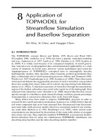
Example 1: Industrial melanism in the peppered moth
Wallace (1858) hypothesized that insects that resemble in color the trunks on which they
reside will survive the longest, due to the concealment from predators. The relatively rapid
rise and fall in the frequency of mutation-based melanism in populations (Figure 8.1) that
occurred in parallel on two continents (Europe, North America), is a compelling example
for rapid microevolution in nature caused by mutation and natural selection. The hypothe-
sis that birds were selectively eating conspicuous insects in habitats modified by industrial
fallout is consistent with the data (Majerus, 1998; Cook, 2000; Coyne, 2002; Grant, 2002).
Example 2: Warning coloration and mimicry
In his famous book, Wallace (1889) devoted a comprehensive chapter to the topic “warn-
ing coloration and mimicry with special reference to the Lepidoptera”. One of the most
conspicuous day-flying moths in the Eastern tropics was the widely distributed species
Opthalmis lincea (Agaristidae). These brightly colored moths have developed chemical
repellents that make them distasteful, saving them from predation (Miillerian mimetics).
O. lincea (Figure 8.2A) is mimicked by the moth Artaxa simulans (Liparidae), which was
collected during the voyage of the Challanger and later described as a new species
(Figure 8.2B). This survival mechanism is called Batesian mimetics (Kettlewell, 1965).
170
A New Ecology: Systems Perspective
Else_SP-Jorgensen_ch008.qxd 3/29/2007 09:59 Page 170
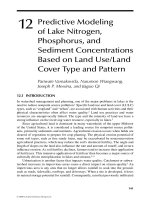
Example 3: Darwin’s finches

Darwin’s finches exemplify the way one species’ gene pools have adapted for long-term
survival via their offspring. The Darwin’s finches diagram below illustrates the way the
finch has adapted to take advantage of feeding in different ecological niches (Figure 8.3).
Their beaks have evolved over time to be best suited to their feeding situation. For
example, the finches that eat grubs have a thin extended beak to poke into holes in the
ground and extract the grubs. Finches that eat buds and fruit would be less successful at
doing this, while their claw like beaks can grind down their food and thus give them a
selective advantage in circumstances where buds are the only real food source for finches.
Example 4: The role of size in horses’ lineage
Maybe the horses’ lineage offers one of the best-known illustrations regarding the role of
size, profoundly documented through a very well-known fossil record. In the early Eocene
(50–55million years ago), the smallest species of horses’ ancestors had approximately the
size of a cat, while other species weighted up to 35kg. The Oligocene species, approximately
Chapter 8: Ecosystem principles have broad explanatory power in ecology
171
form: typica form: carbonaria
s
p
ecies: Biston betularia
AB
Figure 8.1 Industrial melanism in populations of the peppered moth (Biston betularia).
Previously to 1850, white moths peppered with black spots (typica) were dominant in England (A).
Between 1850 and 1920, as a response to air pollution that accompanied the rise of heavy indus-
try, typica was largely replaced by a black form (carbonaria) (B), produced by a single allele, since
dark moths are protected from predation by birds. Between 1950 and 1995, this trend reversed,
making form (B) rare and (A) again common. (Adapted from Kettlewell, 1965).
Ophtalmis lincea
A
Artaxa Simulans
B

Figure 8.2 Insects have evolved highly efficient survival mechanisms that were described in
detail by A.R. Wallace. One common moth species (Opthalmis lincea) (A) contains chemical
repellents to make the insects distasteful. This moth is mimicked by a second species (Artaxa sim-
ulans) (B) From Wallace (1889).
Else_SP-Jorgensen_ch008.qxd 3/29/2007 09:59 Page 171
30million years ago, were bigger, probably weighing up to approximately 50kg. In the
middle Miocene, approximately 17–18 million years ago, grazing “horses” of the size up to
100kg were normal. Numerous fossils have shown that the weight reached approximately
200kg 5million years ago and approximately 500kg 20,000 years ago. Why did this increase
in size offer a selective advantage?
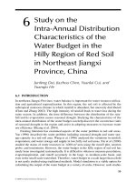
Figure 8.4 shows a model in form of a STELLA diagram that has been used to answer
this question. The model equations are shown in Table 8.1.
The model has been used to calculate the efficiency for different maximum weights.
Heat loss is proportional to weight to the exponent 0.75 (Peters, 1983). The growth rate
follows also the surface, but the growth rate is proportional to the weight to the exponent
0.67 (see equations in Table 8.1). The results are shown in Table 8.2 and the conclusion
is clear: the bigger the maximum weight, the better the eco-exergy efficiency. This is of
course not surprising because a bigger weight means that the specific surface that deter-
mines the heat loss by respiration decreases. As the respiration loss is the direct loss of
free energy, relatively more heat is lost when the body weight is smaller. Notice that the
maximum size is smaller than the supper maximum size that is a parameter to be used in
the model equations (see also Table 8.2).
The evolutionary theory at the light of ecosystem principles
Although living systems constitute very complex systems, they obviously comply with
physical laws (although they are not entirely determined by them), and therefore in
ecological theory it should be checked that each theoretical explanation conforms to
basic laws of physics. First, one needs to understand the implications of the three gen-
erally accepted laws of thermodynamics in terms of understanding organisms’ behavior
and ecosystems’ function. Nevertheless, although the three laws of thermodynamics are
effective in describing system’s behavior close to the thermodynamic equilibrium, in far

from equilibrium systems, such as ecosystems, it has been recognized that although the
172
A New Ecology: Systems Perspective
Beaks adaptive radiation
Large Ground
Finch
Medium Ground
Finch
Small Ground
Finch
Vegetarian
Finch
Large Tree
Finch
Small Tree
Finch
Woodpeeker
Finch
Warbler
Finch
Cactus
Finch
Sharp-Billed
Ground
Finch
Mainly
Animal
Food
Mainly
Plant

Food
Original Finch
Warbler
Cocos
V
egetarian
Small tree
Sharp Beaked
Ground
Medium Tree
Cactus
Large Tree
Large Cactus
Mangrove
Woodpecker
Small Ground
Medium Ground
Large Ground
Figure 8.3 Darwin’s finches diagram.
Else_SP-Jorgensen_ch008.qxd 3/29/2007 09:59 Page 172
three basic laws remain valid, they represent an incomplete picture when describing
ecosystem functioning. This is the purpose of “irreversible thermodynamics” or “non-
equilibrium thermodynamics”. A tentative Ecological Law of Thermodynamics was
proposed by Jørgensen (1997) as: If a system has a through-flow of Exergy, it will attempt
to utilize the flow to increase its Exergy, moving further away from thermodynamic
Chapter 8: Ecosystem principles have broad explanatory power in ecology
173
org
growth
respiration

total food
food eff
consumption
Graph1
Table1
Figure 8.4 The growth and respiration follow allometric principles (Peters, 1983). The growth
equation describes logistic growth with a maximum weight. The food efficiency is found as a result
of the entire life span, using the -values for mammals and grass (mostly Gramineae). The equa-
tions are shown in Table 8.1.
Table 8.1 Model equations
d(org(t))/dtϭ(growth–respiration)
INIT orgϭ1kg
INFLOWS: growth ϭ 3 ϫ org
(0.67)
ϫ (1–org/upper maximum size)
OUTFLOWS: respirationϭ0.5ϫorg
(3/4)
d(total_food(t))/dtϭ (consumption)
INIT total_foodϭ 0
INFLOWS: consumptionϭgrowth ϩ respiration
food_eff %ϭ2127ϫ100ϫorg(t)/(200ϫ total_food(t))
Note: See the conceptual diagram Figure 8.4.
Else_SP-Jorgensen_ch008.qxd 3/29/2007 09:59 Page 173
equilibrium; If more combinations and processes are offered to utilize the Exergy flow,
the organization that is able to give the highest Exergy under the prevailing circum-
stances will be selected. This hypothesis may be reformulated, as proposed by de Wit
(2005) as: If a system has a throughflow of free energy, in combination with the evolu-
tionary and historically accumulated information, it will attempt to utilize the flow to
move further away from the thermodynamic equilibrium; if more combinations and
processes are offered to utilize the free energy flow, the organization that is able to give

the greatest distance away from thermodynamic equilibrium under the prevailing cir-
cumstances will be selected.
Both formulations mean that to ensure the existence of a given system, a flow of
energy, or more precisely Exergy, must pass through it, meaning that the system cannot
be isolated. Exergy may be seen as energy free of entropy (Jørgensen, 1997; Jørgensen
and Marques, 2001), i.e. energy which can do work. A flow of Exergy through the sys-
tem is sufficient to form an ordered structure, or dissipative structure (Prigogine, 1980).
If we accept this, then a question arises: which ordered structure among the possible ones
will be selected or, in other words, which factors influence how an ecosystem will grow
and develop? The difference between the formulation by exergy or eco-exergy and free
energy has been discussed in Chapter 6.
Jørgensen (1992b, 1997) proposed a hypothesis to interpret this selection, providing
an explanation for how growth of ecosystems is determined, the direction it takes, and its
implications for ecosystem properties and development. Growth may be defined as the
increase of a measurable quantity, which in ecological terms is often assumed to be the
biomass. But growth can also be interpreted as an increase in the organization of ordered
structure or information. From another perspective, Ulanowicz (1986) makes a distinc-
tion between growth and development, considering these as the extensive and intensive
aspects, respectively, of the same process. He argues that growth implies increase or
expansion, while development involves increase in the amount of organization or infor-
mation, which does not depend on the size of the system.
According to the tentative Ecological Law of Thermodynamics, when a system grows
it moves away from thermodynamic equilibrium, dissipating part of the Exergy in cata-
bolic processes and storing part of it in its dissipative structure. Exergy can be seen as a
measure of the maximum amount of work that the ecosystem can perform when it is
174
A New Ecology: Systems Perspective
Table 8.2 Eco-exergy efficiency for the life span for different maximum sizes
a
Maximum size Eco-exergy efficiency Upper maximum size parameter

(kg) (percent) (kg)
35 1.41 45
50 1.55 65
100 1.84 132
200 2.20 268
500 2.75 690
a
-Value for mammals is 2127 and for grass is 200.
Else_SP-Jorgensen_ch008.qxd 3/29/2007 09:59 Page 174
brought into thermodynamic equilibrium with its environment. In other words, if an
ecosystem were in equilibrium with the surrounding environment its exergy would be
zero (no free energy), meaning that it would not be able to produce any work, and that all
gradients would have been eliminated.
Structures and gradients, resulting from growth and developmental processes, will be
found everywhere in the universe. In the particular case of ecosystems, during ecological
succession, exergy is presumably used to build biomass, which is exergy storage. In other
words, in a trophic network, biomass, and exergy will flow between ecosystem compart-
ments, supporting different processes by which exergy is both degraded and stored in dif-
ferent forms of biomass belonging to different trophic levels.
Biological systems are an excellent example of systems exploring a plethora of possi-
bilities to move away from thermodynamic equilibrium, and thus it is most important in
ecology to understand which pathways among the possible ones will be selected for
ecosystem development. In thermodynamic terms, at the level of the individual organism,
survival and growth imply maintenance and increase of the biomass, respectively.
From the evolutionary point of view, it can be argued that adaptation is a typically self-
organizing behavior of complex systems, which may explain why evolution apparently
tends to develop more complex organisms. On one hand, more complex organisms have
more built-in information and are further away from thermodynamic equilibrium than
simpler organisms. In this sense, more complex organisms should also have more stored
exergy (thermodynamic information) in their biomass than the simpler ones. On the other

hand, ecological succession drives from more simple to more complex ecosystems, which
seem at a given point to reach a sort of balance between keeping a given structure, emerg-
ing for the optimal use of the available resources, and modifying the structure, adapting it
to a permanently changing environment. Therefore, an ecosystem trophic structure as a
whole, there will be a continuous evolution of the structure as a function of changes in the
prevailing environmental conditions, during which the combination of the species that
contribute the most to retain or even increase exergy storage will be selected.
This constitutes actually a translation of Darwin’s theory into thermodynamics
because survival implies maintenance of the biomass, and growth implies increase in bio-
mass. Exergy is necessary to build biomass, and biomass contains exergy, which may be
transferred to support other exergy (energy) processes.
The examples of industrial melanism in the peppered moth and warning coloration
and mimicry are compliant with the Ecological Law of Thermodynamics, illustrating at
the individual and population levels how the solutions able to improve survival and main-
tenance or increase in biomass under the prevailing conditions were selected. Also, the
adaptations of Darwin’s finches to take advantage of feeding in different ecological
niches constitute another good illustration at the individual and population levels.
Depending on the food resources available at each niche, the beaks evolved throughout
time to be best suited to their function in the prevailing conditions, improving survival,
and biomass growth capabilities. Finally, the horses’ lineage increase in size illustrates
very well how a bigger weight determines a decrease in body specific surface and con-
sequently a decrease in the direct loss of free energy (heat loss by respiration). From the
thermodynamic point of view, we may say that the solutions able to give the highest
Chapter 8: Ecosystem principles have broad explanatory power in ecology
175
Else_SP-Jorgensen_ch008.qxd 3/29/2007 09:59 Page 175
exergy under the prevailing circumstances were selected, maintaining or increasing gra-
dients and therefore keeping or increasing the distance to thermodynamic equilibrium.
8.3 DO ECOLOGICAL PRINCIPLES ENCOMPASS OTHER PROPOSED
ECOLOGICAL THEORIES?: ISLAND BIOGEOGRAPHY

In the next section, we consider another important ecological theory, namely island bio-
geography. Why do many more species of birds occur on the island of New Guinea than
on the island of Bali? One answer is that New Guinea has more than 50 times the area of
Bali, and numbers of species ordinarily increase with available space. This does not, how-
ever, explain why the Society Islands (Tahiti, Moorea, Bora Bora, etc.), which collec-
tively have about the same area as the islands of the Louisiade Archipelago off New
Guinea, play host to much fewer species, or why the Hawaiian Islands, ten times the area
of the Louisiades, also have fewer native birds.
Two eminent ecologists, the late Robert MacArthur of Princeton University and E.O.
Wilson of Harvard, developed a theory of “island biogeography” to explain such uneven
distributions (MacArthur and Wilson, 1967). They proposed that the number of species
on any island reflects a balance between the rate at which new species colonize it and the
rate at which populations of established species become extinct (Figure 8.5). If a new vol-
canic island were to rise out of the ocean off the coast of a mainland inhabited by 100
species of birds, some birds would begin to immigrate across the gap and establish pop-
ulations on the empty, but habitable, island. The rate at which these immigrant species
could become established, however, would inevitably decline, for each species that suc-
cessfully invaded the island would diminish by one the pool of possible future invaders
(the same 100 species continue to live on the mainland, but those which have already
become residents of the island can no longer be classed as potential invaders).
Equally, the rate at which species might become extinct on the island would be related
to the number that had become residents. When an island is nearly empty, the extinction
rate is necessarily low because few species are available to become extinct. And since the
resources of an island are limited, as the number of resident species increases, the smaller
176
A New Ecology: Systems Perspective
Number of s
p
ecies Number of s
p

ecies
Number of species
going extinct per year
Number of new species
arriving per year
EXTINCTION CURVE IMMIGRATION CURVE
Figure 8.5 Extinction and immigration curves.
Else_SP-Jorgensen_ch008.qxd 3/29/2007 09:59 Page 176
and more extinction prone their individual populations are likely to become. The rate at
which additional species will establish populations will be high when the island is
relatively empty, and the rate at which resident populations go extinct will be high when
the island is relatively full. Thus, there must be a point between 0 and 100 species (the
number on the mainland) where the two rates are equal, and therefore the input from
immigration balances output from extinction. That equilibrium in the number of species
(Figure 8.6) would be expected to remain constant as long as the factors determining the
two rates did not change. But the exact species present should change continuously as
some species go extinct and others invade (including some that have previously gone
extinct), so that there is a steady turnover in the composition of the fauna.
Examples
Example 1: Krakatau Island
One famous “test” of the theory was provided in 1883 by a catastrophic volcanic explo-
sion that devastated the island of Krakatau, located between the islands of Sumatra and
Java. The flora and fauna of its remnant and of two adjacent islands were completely exter-
minated, yet within 25 years (1908) 13 species of birds had re-colonized what was left of
the island. By 1919–1921 28-bird species were present, and by 1932–1934, 29. Between
the explosion and 1934, 34 species actually became established, but five of them went
extinct. By 1951–1952 33 species were present, and by 1984–1985, 35 species. During
this half century (1934–1985), a further 14 species had become established, and 8 had
become extinct. As the theory predicted, the rate of increase declined as more and more
species colonized the island. In addition, as equilibrium was approached there was some

turnover. The number in the cast remained roughly the same while the actors gradually
changed.
The theory predicts other things, too. For instance, everything else being equal, distant
islands will have lower immigration rates than those close to a mainland, and equilibrium
Chapter 8: Ecosystem principles have broad explanatory power in ecology
177
Number of s
p
ecies
EXT Curve
IMMIG Curve
S
Figure 8.6 The equilibrium number of species. Any particular island has a point where the
extinction (EXT curve) and immigration curves (IMMIG curve) intersect. At this point the num-
ber of new immigrating species to the island is exactly matched by the rate at which species are
going extinct.
Else_SP-Jorgensen_ch008.qxd 3/29/2007 09:59 Page 177
will occur with fewer species on distant islands (Figure 8.7). Close islands will have high
immigration rates and support more species. By similar reasoning, large islands, with
their lower extinction rates, will have more species than small ones—again everything
else being equal (which frequently is not, for larger islands often have a greater variety
of habitats and more species for that reason).
Island biogeography theory has been applied to many problems, including forecasting
faunal changes caused by fragmenting previously continuous habitat. For instance, in
most of the eastern United States only patches of the once-great deciduous forest remain,
and many species of songbirds are disappearing from those patches. One reason for the
decline in birds, according to the theory, is that fragmentation leads to both lower immi-
gration rates (gaps between fragments are not crossed easily) and higher extinction rates
(less area supports fewer species).
Example 2: Connecticut forest re-establishing

Indications of such changes in species composition during habitat fragmentation were
found in studies conducted between 1953 and 1976 in a 16-acre nature preserve in
Connecticut in which a forest was re-establishing itself. During that period development
was increasing the distance between the preserve and other woodlands. As the forest grew
back, species such as American Redstarts that live in young forest colonized the area, and
birds such as the Field Sparrow, which prefer open shrub lands, became scarce or disap-
peared. In spite of the successional trend toward large trees, however, two bird species
normally found in mature forest suffered population declines, and five such species went
extinct on the reserve. The extinctions are thought to have resulted from lowering immi-
gration rates caused by the preserve’s increasing isolation and by competition from six
invading species characteristic of suburban habitats.
178
A New Ecology: Systems Perspective
Number of Species Number of Species
S
S
CLOSER ISLANDS MORE DISTANT ISLANDS
EXT Curve EXT Curve
IMMIG Curve IMMIG Curve
Figure 8.7 The influence of distance of an island from the source on the equilibrium number of
species. EXT curve, Extinction curve. IMMIG curve, Immigration curve.
Else_SP-Jorgensen_ch008.qxd 3/29/2007 09:59 Page 178
Example 3: Bird community in an oak wood in Surrey, England
Long-term studies of a bird community in an oak wood in Surrey, England, also support
the view that isolation can influence the avifauna of habitat islands. A rough equilibrium
number of 32 breeding species were found in that community, with a turnover of three
additions and three extinctions annually. It was projected that if the woods were as thor-
oughly isolated as an oceanic island, it would maintain only five species over an extended
period: two species of tits (same genus as titmice), a wren, and two thrushes (the English
Robin and Blackbird).

Island biogeography theory can be a great help in understanding the effects of habitat
fragmentation. It does not, however, address other factors that can greatly influence which
birds reside in a fragment. Some of these include whether nest-robbing species are pres-
ent in such abundance that they could prevent certain invaders from establishing them-
selves, whether the fragment is large enough to contain a territory of the size required by
some members of the pool of potential residents, or whether other habitat requirements of
species in that pool can be satisfied. To take an extreme example of the latter, Acorn,
Nuttall’s, Downy, or Hairy Woodpeckers would not colonize a grass-covered, treeless habi-
tat in California, even if they were large, and all four woodpeckers are found in adjacent
woodlands.
Island biogeography theory at the light of ecosystem principles
In general terms, the Island Biogeography Theory explains therefore why, if everything
else is similar, distant islands will have lower immigration rates than those close to a
mainland, and ecosystems will contain fewer species on distant islands, while close
islands will have high immigration rates and support more species. It also explains why
large islands, presenting lower extinction rates, will have more species than small ones.
This theory forecasts effect of fragmenting previously continuous habitat, considering
that fragmentation leads to both lower immigration rates (gaps between fragments are not
crossed easily) and higher extinction rates (less area supports fewer species).
The Ecological Law of Thermodynamics equally provides a sound explanation for the
same observations. Let us look in first place to the problem of the immigration curves. In
all the three examples, the decline in immigration rates as a function of increasing isolation
(distance) is fully covered the concept of openness introduced by Jørgensen (2000a). Once
accepted the initial premise that an ecosystem must be open or at least non-isolated to be
able to import the energy needed for its maintenance, islands’ openness will be inversely
proportional to its distance to mainland. As a consequence, more distant islands have lower
possibility to exchange energy or matter and decreased chance for information inputs,
expressed in this case as immigration of organisms. The same applies to fragmented habi-
tats, the smaller the plots of the original ecosystem the bigger the difficulty in recovering
(or maintaining) the original characteristics. After a disturbance, the higher the openness the

faster information and network (which may express as biodiversity) recovery will be.
The fact that large islands present lower extinction rates and more species than small
ones, as well as less fragmented habitats in comparison with more fragmented ones, also
complies with the Ecological Law of Thermodynamics. All three examples can be inter-
preted in this light. Actually, provided that all the other environmental are similar, larger
Chapter 8: Ecosystem principles have broad explanatory power in ecology
179
Else_SP-Jorgensen_ch008.qxd 3/29/2007 09:59 Page 179
islands offer more available resources. Under the prevailing circumstances, solutions able
to give the highest exergy will be selected, increasing the distance to thermodynamic equi-
librium not only in terms of biomass but also in terms of information (i.e. network and bio-
diversity). Moreover, after a disturbance, like in the case of the Krakatau Island, the rate
of re-colonization and ecosystem recovery will be a function of system’s openness.
8.4 DO ECOLOGICAL PRINCIPLES ENCOMPASS OTHER PROPOSED
ECOLOGICAL THEORIES?: LATITUDINAL GRADIENTS IN
BIODIVERSITY
On a global scale, species diversity typically declines with increasing latitude toward the
poles (Rosenzweig, 1995; Stevens and Willig, 2002). Although the latitude diversity gra-
dient is the most striking biodiversity pattern, the dynamics that generate and maintain
this trend remain poorly understood. The latitudinal diversity gradient is commonly
viewed as the net product of in situ origination and extinction, with the tropics serving as
either a generator of biodiversity (the tropics-as-a-cradle hypothesis), or an accumulator
of biodiversity (the tropics-as-museum hypothesis), eventually both.
The causes for latitudinal gradients in biodiversity (o/gradients-
biodiversity.htm).
The determinant of biological diversity is not latitude per se, but the environmental
variables correlated with latitude. More than 25 different mechanisms have been sug-
gested for generating latitudinal diversity gradients, but no consensus has been reached
yet (Gaston, 2000).
One factor proposed as a cause of latitudinal diversity gradients is the area of the cli-

matic zones. Tropical landmasses have a larger climatically similar total surface area than
landmasses at higher latitudes with similarly small temperature fluctuations
(Rosenzweig, 1992). This may be related to higher levels of speciation and lower levels
of extinction in the tropics (Rosenzweig, 1992; Gaston, 2000; Buzas et al., 2002).
Moreover, most of the land surface of the Earth was tropical or subtropical during the
Tertiary, which could in part explain the greater diversity in the tropics today as an out-
come of historical evolutionary processes (Ricklefs, 2004).
The higher solar radiation in the tropics increases productivity, which in turn is
thought to increase biological diversity. However, productivity can only explain why there
is more total biomass in the tropics, not why this biomass should be allocated into more
individuals, and these individuals into more species (Blackburn and Gaston, 1996). Body
sizes and population densities are typically lower in the tropics, implying a higher number
of species, but the causes and the interactions among these three variables are complex
and still uncertain (Blackburn and Gaston, 1996).
Higher temperatures in the tropics may imply shorter generation times and greater
mutation rates, thus accelerating speciation in the tropics (Rohde, 1992). Speciation may
also be accelerated by a higher habitat complexity in the tropics, although this does not
apply to freshwater ecosystems. The most likely explanation is a combination of various
factors, and it is expected that different factors affect differently different groups of
organisms, regions (e.g. northern vs. southern hemisphere) and ecosystems, yielding the
variety of patterns that we observe.
180
A New Ecology: Systems Perspective
Else_SP-Jorgensen_ch008.qxd 3/29/2007 09:59 Page 180
Examples
Example 1: Geographic range of marine prosobranch gastropods
Roy et al. (1998) have assembled a database of the geographic ranges of 3916 species of
marine prosobranch gastropods living in waters shallower than 200 m of the western
Atlantic and eastern Pacific Oceans, from the tropics to the Artic Ocean. They have found
that Western Atlantic and eastern Pacific diversities were similar, and that the diversity

gradients were strikingly similar despite many important physical and historical differ-
ences between the oceans. Figure 8.8 shows the strong latitudinal diversity gradients that
are present in both oceans.
The authors have found that one parameter that did correlate significantly with diver-
sity in both oceans was solar energy input, as represented by average sea surface temper-
ature. More, the authors continued saying that if that correlation was causal, sea surface
temperature is probably linked to diversity through some aspect of productivity. They
defend that if that is the case, diversity is an evolutionary outcome of trophodynamics
processes inherent in ecosystems, and not just a by-product of physical geographies.
Example 2: Latitudinal trends in vertebrate diversity ( />Amphibians, absent from arctic regions, are well represented in the mid-latitudes
(Figure 8.9A). Forty-seven species of amphibians are found in California (Laudenslayer and
Grenfell, 1983). As might be expected given the warmth and humidity of much of the trop-
ics and the inability of amphibians to thermoregulate, this group reaches its greatest diversity
here. In fact, one of the three orders (groups of related families) of the class Amphibia, called
caecilians (160 species of worm-like creatures), is restricted in its distribution to the tropics.
Chapter 8: Ecosystem principles have broad explanatory power in ecology
181
1000
800
600
400
200
0
-10 0 10 20 30 40 50 60 70 80 9
0
W.Atlantic
E.Pacific
No. of species
Latitude
(

de
g
rees
)
Figure 8.8 Latitudinal diversity gradient of eastern Pacific and western Atlantic marine proso-
branch gastropods, binned per degree of latitude. The range of a species is assumed to be contin-
uous between its range endpoints, so diversity for any given latitude is defined as the number of
species whose latitudinal ranges cross that latitude.
Else_SP-Jorgensen_ch008.qxd 3/29/2007 09:59 Page 181
Reptiles, too, are represented by more species in the temperate latitudes. The diversity
of lizards is shown in Figure 8.9B and for snakes is shown in Figure 8.9C. Both of these
figures show slight decreases in diversity for these groups between 15 and 30Њ latitude.
These are the latitudes at which most of the world’s deserts are found. There are 77
species of reptiles in California (Laudenslayer and Grenfell, 1983). The two major groups
of terrestrial reptiles, lizards and snakes, are represented by more species in the tropics
than in higher latitudes. The pattern is even more pronounced for turtles.
Birds really increase in diversity in temperate latitudes. For example, at least 88-bird
species breed on the Labrador Peninsula of northern Canada (55Њ N), 176 species breed
in Maine (45Њ N), and more than 300 species can be found in Texas (31Њ N; Peterson,
1963). The total number of bird species found in California exceeds 540 (Laudenslayer
and Grenfell, 1983); the total for all of North America is roughly 700 (Welty, 1976).
An indication of the latitudinal trend in mammalian diversity was provided by
Simpson (1964) for continental North American mammals. Here again, species diversity
is apparent with decreasing latitude. This analysis also shows that, superimposed on the
latitudinal trend, is an effect due to elevation such that mountainous regions have more
species of mammals than lowlands. There are 214 species of mammals in California
(Laudenslayer and Grenfell, 1983).
A majority of all fish species are found in tropical waters. It is possible to get an indi-
cation of the diversity of fish in the tropics by considering two examples, one freshwater
182

A New Ecology: Systems Perspective
No. of units in taxon employed
LatitudeLatitude LatitudeNNSS
AC
90
1
2
3
4
6
8
20
40
100
80
60
90 90 9060 60 60 60 606030 30 30 30 30 3000
0
NS
B
Figure 8.9 Diversity vs. latitude plots for three groups of terrestrial poikilotherms, showing what
appear to be latitude-related anomalies in the region 15–30Њ that are probably a response to the less
favorable conditions prevailing in the desert regions often found in those latitudes. Data show the
highest number of genera in 5Њ latitude classes. Solid curve smoothed through points indicating
highest diversity, dotted curve following the points suggestive of persistent anomaly. (A) Genera
of amphibians. (B) Genera of lizards. (C) Genera of snakes.
Else_SP-Jorgensen_ch008.qxd 3/29/2007 09:59 Page 182
and one marine. The first example is provided by the dazzling array of coral reef fish.
Something on the order of 30–40% of all marine fish species are in some way associated
with tropical reefs and more than 2200 species can be found in a large reef complex

(Moyle and Cech, 1996). Second, the Amazon River of South America, huge in compa-
rison to most other river systems—3700 miles long, drains a quarter of the South
American continent—has over 2400 species of fish. The Rio Negro, a tributary of the
Amazon, contains more fish species than all the rivers of the United States combined.
Example 3: Trends within plant communities and across latitude
Niklas et al. (2003) examined how species richness and species-specific plant density—
number of species and number of individuals per species, respectively—vary within com-
munity size frequency distributions and across latitude. 226 forested plant communities from
Asia, Africa, Europe, and North, Central, and South America were studied (60Њ4ЈN–41Њ4ЈS)
using the Gentry database. An inverse latitudinal relationship was observed between species
richness and species-specific plant density. Their analyses showed that the species richness
increased toward the tropics and the reverse trend was observed for average species-specific
plant density.
Example 4: Trends within marine epifaunal invertebrate communities
Witman et al. (2004) tested the effects of latitude and the richness of the regional pool on
the species richness of local epifauna invertebrate communities by sampling the diversity
of local sites in 12-independent biogeographic regions from 62ЊS to 63ЊN. Both regional
and local species richness displayed significant unimodal patterns with latitude, peaking
at low latitudes and decreasing toward high latitudes (Figure 8.10).
Latitudinal gradients in biodiversity at the light of ecosystem principles
Latitudinal gradients in biodiversity are easily interpretable at the light of the Ecological
Law of Thermodynamics. Obviously, the higher solar radiation in the tropics increases
productivity, which in turn is thought to increase biological diversity. In fact, Blackburn
and Gaston (1996) found that one parameter that did correlate significantly with diver-
sity in both oceans was solar energy input, as represented by average sea surface tem-
perature. Moreover, these authors claim that if that correlation was causal, sea surface
temperature is probably linked to diversity through some aspect of productivity. However,
they could not establish the causal nexus, considering that productivity could only
explain why there is more total biomass in the tropics, not why this biomass should be
allocated into more individuals, and these individuals into more species.

This apparent inconsistency can nevertheless be explained within the frame of ecosys-
tem principles. In fact, Jørgensen et al. (2000), proposed that ecosystems show three
growth forms:
I. Growth of physical structure (biomass), which is able to capture more of the incom-
ing energy in the form of solar radiation but also requires more energy for mainte-
nance (respiration and evaporation).
II. Growth of network, which means more cycling of energy or matter.
Chapter 8: Ecosystem principles have broad explanatory power in ecology
183
Else_SP-Jorgensen_ch008.qxd 3/29/2007 09:59 Page 183
III. Growth of information (more developed plants and animals with more genes), from
r-strategists to K-strategists, which waste less energy but also usually carry more
information.
This was experimentally confirmed by Debeljak (2002) examining managed and virgin
forest in different development stages (e.g. pasture, gap, juvenile, optimum forest).
Accordingly, these three growth forms may be considered an integration of Odum’s
attributes, which describe changes in ecosystems associated with development from the
early stage to the mature stage. Clearly, Blackburn and Gaston (1996) were considering
only growth form I.
8.5 DO ECOLOGICAL PRINCIPLES ENCOMPASS OTHER PROPOSED
ECOLOGICAL THEORIES?: OPTIMAL FORAGING THEORY
Researchers have long pursued theories to explain species’ diversity. These theories have
focused on quantifying adaptation, fitness, and natural selection through observing an
animal’s feeding behaviors. The assumption is that feeding behaviors are reflections of
these internal processes. Using behavior as a mechanism of adaptation in a feedback loop
creates an interactive system between an animal’s phenotype and its environment.
184
A New Ecology: Systems Perspective
AB
C

0
50
-80 -60 -40 -20 0
Latitude
20 40 60 80
-80 -60 -40 -20 0
Latitude
20 40 60 80 -80 -60 -40 -20 0
Latitude
20 40 60 80
100
150
350
200
250
300
Local species
richness (S
obs.
)
0
200
400
600
800
1000
1200
1400
Number of species
in region

0
50
100
150
200
350
300
250
Local species
richness (Chao 2)
Figure 8.10 Species richness as a function of latitude. (A) Regional species richness (standard
regional pool). (B) Local species richness based on the Chao2 estimate. (C) Local species richness
as S
obs
. Lines represent significant, best fits to second-order polynomial equations.
Else_SP-Jorgensen_ch008.qxd 3/29/2007 09:59 Page 184
MacArthur and Pianka (1966) first proposed an optimal foraging theory, arguing that
because of the key importance of successful foraging to an individual’s survival, it should
be possible to predict foraging behavior by using decision theory to determine the behav-
ior that would be shown by an “optimal forager”—one with perfect knowledge of what
to do to maximize usable food intake. In their paper, a graphical model of animal feed-
ing activities based on costs versus profits was developed. A forager’s optimal diet was
specified and some interesting predictions emerged. Prey abundance influenced the
degree to which a consumer could afford to be selective because it affected search time
per item eaten. Diets should be broad when prey are scarce (long search time), but nar-
row if food is abundant (short search time) because a consumer can afford to bypass infe-
rior prey only when there is a reasonably high probability of encountering a superior item
in the time it would have taken to capture and handle the previous one. Also, larger
patches should be used in a more specialized way than smaller patches because travel
time between patches (per item eaten) is lower.

Succinctly, this heavily referenced paper in evolutionary biology presented three concepts:
(1) How long a predator will forage in a specific area?
(2) Influence of prey density on the length of time a predator will forage in an area.
(3) Influence of prey variety on a predator’s choice of acquired prey.
These concepts describe a predator’s behavior as a function of its relationship with the
prey it acquires. Fundamental conditions in these concepts influencing the predator–prey
relationship are time foraging and prey availability. Within these concepts, MacArthur
and Pianka embodied the study of differential land and resource use in a specific field of
study: optimal foraging theory.
Examples
Example 1: Rufous Hummingbirds
Carpenter et al. (1983) found a way to test optimal foraging theory, using Rufous
Hummingbirds. These hummers establish feeding territories during stops on their 2000-
mile migration between their breeding grounds in the Pacific Northwest and their win-
tering habitat in southern Mexico. They zealously guard those territories, driving off
hawkmoths, butterflies, other hummers, and even bees that might compete for the nectar.
In addition, they deplete the nectar resources around the periphery of their territories as
early in the day as they can, in order to out-compete other nectar-sippers that might try
to sneak a drink at the territory edge.
When half of the flowers in a territory were covered with cloth so the birds could not
drain them, Carpenter and her co-workers found that the resident hummer increased its
territory size. This showed that territoriality was tied to the availability of nectar, and that
the bird could in some way assess the amount of nectar it controlled. Then, by substitut-
ing a sensitive scale topped by a perch for the territory-holder’s traditional perch, they
were able to measure the bird’s weight each time it alighted. The researchers found that
the hummers optimized their territory size by trial and error, making it larger or smaller
Chapter 8: Ecosystem principles have broad explanatory power in ecology
185
Else_SP-Jorgensen_ch008.qxd 3/29/2007 09:59 Page 185
until their daily weight gain was at a maximum. In this case of migrant-territorial hum-

mers, theory accurately predicted how a bird behaves in nature.
Example 2: Optimal clam selection by northwestern crows (Alcock, 1997)
Richardson and Verbeek (1986) noticed that crows in the Pacific Northwest often leave lit-
tleneck clams uneaten after locating them. The crows dig the clams from their burrows, but
they often leave the smaller ones on the beach and only bother with the larger ones, which
they drop on the rocks and eat. Their acceptance rate increases with prey size: they open and
eat only about half of the 29-mm-long clams they find, while consuming all clams in the
32–33 mm range. The two researchers determined that the most profitable clams were the
largest, not because they broke more easily, but because they contained more calories than
smaller clams. By considering the caloric benefits from clams of different sizes and the costs
of searching for, digging up, opening, and feeding on clams, the authors were able to con-
struct a mathematical model based on the assumption that crows would select an optimal
diet, in this case one that maximized their caloric intake. The model predicted that clams
approximately 28.5 mm in length would be opened and eaten half the time, given the search
costs required to find clams of different sizes; the crows behavior shows that they agree with
researchers’ match (Figure 8.11). Their work was based on optimal foraging theory.
The optimal foraging theory at the light of ecosystem principles
The optimal foraging theory clearly complies with the Ecological Law of
Thermodynamics. The fact that prey abundance influences consumers’ selectivity and
that diets are broad when prey are scarce and narrow if food is abundant, as a function of
search for food time, is clearly translated by “… If more combinations and processes are
186
A New Ecology: Systems Perspective
100
50
25.0
Clam length (mm)
35.0
Percentage eaten
Figure 8.11 Optimality model of prey selection in relation to prey size. The curve represents the

predicted percentages of small to large clams that crows should select for consumption after locat-
ing, based on the assumption that the birds attempt to maximize the rate of energy gain per unit of
time spent foraging for clams. The solid circles represent the actual observations, showing the
model’s predictions were supported (Richardson and Verbeek, 1986).
Else_SP-Jorgensen_ch008.qxd 3/29/2007 09:59 Page 186
offered to utilize the Exergy flow, the organization that is able to give the highest Exergy
under the prevailing circumstances will be selected or by if more combinations and
processes are offered to utilize the free energy flow, the organization that is able to give
the greatest distance away from thermodynamic equilibrium under the prevailing cir-
cumstances will be selected ”. Both examples can, therefore, be easily explained by the
same ecosystem principles.
8.6 DO ECOLOGICAL PRINCIPLES ENCOMPASS OTHER PROPOSED
ECOLOGICAL THEORIES?: NICHE THEORY
Hutchinson (1957, 1965) suggested that an organism’s niche could be visualized as a
multidimensional space, or hypervolume, formed by the combination of gradients of each
single environmental condition to which the organism was exposed. The N-environmental
exposure conditions form a set of N-intersecting axes within which one can define an
N-dimensional niche hypervolume unique to each species. The niche hypervolume is com-
prised of all combinations of the environmental conditions that permit an individual of that
species to survive and reproduce indefinitely (Huthchinson’s Fundamental niche).
Hutchinson distinguished the fundamental niche, defined as the maximum inhabitable
hypervolume in the absence of competition, predation, and parasitism, from the realized
niche, which is a smaller hypervolume occupied when the species is under biotic constraints.
Hutchinson also defined the niche breadth for an organism as the habitable range, between
the maximum and the minimum, for each particular environmental variable. Thus, the niche
breadth is the projection of the niche hypervolume onto each individual environment.
Following Hutchinson’s distinction, niche refers to the requirements of the species and
habitat refers to a physical place in the environment where those requirements can be met
(Figure 8.12).
To interpret Figure 8.12 with regard to the distribution of species 1 and 2, one must

understand Hutchinson’s emphasis on the fundamental importance of competition as a
force influencing the distribution of species in nature. Hutchinson argued that in the face
of competition, a species will not utilize its entire fundamental niche, but rather the real-
ized niche actually used by the species will be smaller, only consisting of those portions
of the fundamental niche where the species is competitively dominant. As a result of
competitive exclusion, according to Hutchinson, the realized niche is smaller than the
fundamental niche, and a species may frequently be absent from portions of its funda-
mental niche because of competition with other species. Obviously, the more limited
resources two populations have in common (i.e. the more similar their niches are), the
greater the impact of competition (all else being equal).
In particular, niche is used to describe and analyze:
(1) Ways in which different species interact (including competition, resource portioning,
exclusion, or coexistence).
(2) Why some species are rare and others abundant.
(3) What determines geographical distribution of a given species?
(4) What determines structure and stability of multi-species communities?
Chapter 8: Ecosystem principles have broad explanatory power in ecology
187
Else_SP-Jorgensen_ch008.qxd 3/29/2007 09:59 Page 187
Consider an extreme case: can two populations occupying the same resource niche coex-
ist in the same environment? ( />If two populations occupy same resource niche, then by definition, they utilize all the
same resources and in the same manner. Common sense tells us there are three possible
outcomes to this situation: (1) share resources more or less equally (neither population
changes niche); (2) one or both populations alters niche to reduce overlap (niche parti-
tioning), and (3) one population loses out completely (competitive exclusion). Which
outcome will occur? Answer from niche theoryϭ 2 or 3, but not 1. This somewhat coun-
terintuitive finding given the formal name of competitive exclusion principle (CEP)
(Gause, 1934) states that no two species can permanently occupy the same niche: either
the niches will differ, or one will be excluded by the other (note: “excluded” here means
replaced by differential population growth, not necessarily by fighting or territoriality),

and has become a central tenet of modern niche theory. Of course, 100% niche overlap
is unlikely if not impossible; but such an extreme case is not necessary for competitive
exclusion or other forms of niche change.
Much theory and research in ecology has focused on predicting what actually happens
when there is niche overlap and competition: when does exclusion result, when coexis-
tence? How much overlap is possible (a question treated by the “theory of limiting
similarity”)? How do environmental fluctuations affect this? Why are some species gen-
eralists, others specialists? Both possible responses to niche competition (competitive
exclusion, and coexistence via reduction in niche overlap) are commonly observed, and
their determinants and features have been studied by three means: lab experiments, field
188
A New Ecology: Systems Perspective
Figure 8.12 Distribution of species 1 and 2.
Else_SP-Jorgensen_ch008.qxd 3/29/2007 09:59 Page 188
observations, and mathematical models or simulations. Competitive exclusion is com-
monly observed when a species colonizes a habitat and out-competes indigenous species—
probably due to absence of parasites and predators adapted to exploit the colonizer (e.g.
introduced placentals vs. indigenous marsupials in Australia). Coexistence through niche
partitioning is rarely observed directly, but can often be inferred from traces left by “the
ghost of competition”. The typical means of doing so is to examine two populations that
overlap spatially, but only partially, and then to compare the niche of each population in the
area of overlap versus the area of non-overlap. In such a case, we often observe that in areas
where competitors coexist, one or both have narrower niche range (e.g. diet breadth) than
in areas where competitor is absent; this is because competition “forces” each competing
population to specialize in those resources—or other niche dimensions—in which it has a
competitive advantage, and conversely to “give up” on those in which the other population
out competes it. Thus, in absence of competitors a given species will often utilize a broader
array of resources, closer to its fundamental niche, than it will in competitor’s presence; this
phenomenon is termed “competitive release”.
When niche shift involves an evolutionary change in attributes (“characteristics”) of

competing populations, it is termed character displacement. This is some of the strongest
evidence for the role of competition in shaping niches because it is unlikely to have alter-
native explanation. A classic example of character displacement is change in length or
shape of beaks in ecologically similar bird species that overlap geographically.
Example 1 of the competitive exclusion principle or Gause’s principle: two spp. of
Paramecium
Gause (1934) placed two species of Paramecium into flasks containing a bacterial culture
that served as food. Thus, in this artificial laboratory system both species of paramecium
were forced to have the same niche. Gause counted the number of Paramecium each day
and found that after a few days (Figure 8.13) one species always became extinct because
it apparently was unable to compete with the other species for the single food resource.
However, extinction is not the only possible result of two species having the same niche. If
two competing species can co-exist for a long period of time, then the possibilities exists that
they will evolve differences to minimize competition; that is, they can evolve different niches.
Chapter 8: Ecosystem principles have broad explanatory power in ecology
189
Figure 8.13 Competition between two laboratory populations of Paramecium with similar
requirements.
Else_SP-Jorgensen_ch008.qxd 3/29/2007 09:59 Page 189
Example 2 of the competitive exclusion principle or Gause’s principle: Geospiza spp.
We can go to Darwin’s finches again to see examples of character displacement on the
Galapagos Islands. Members of the genus Geospiza are wide spread among the islands.
Geospiza fortis, for example, is found alone on Daphne Island, while G. fulginosa is found
alone on Crossman Island. Both ground-feeding birds are about the same size. On Charles
and Chatham Islands, on the other hand, the species co-exist. Although G. fortis is about
the same size as their relatives on Daphne, G. fulginosa is considerably smaller than their
neighbors on Crossman. The shift in size allows the G. fortis to feed on smaller seeds, thus
avoiding competition with the larger G. fortis on Charles and Chatham. This and other
documented cases of character displacement suggest that competition is important in
shaping ecosystems. Displacement is interpreted as evidence of historical competition.

Example 3 of the competitive exclusion principle or Gause’s principle: squirrels in
England ( />The red squirrel (Sciurus vulgaris) is native to Britain but its population has declined due
to competitive exclusion, disease, and the disappearance of hazel coppices and mature
conifer forests in lowland Britain. The grey squirrel (Sciurus carolinensis) was introduced
to Britain in approximately 30 sites between 1876 and 1929. It has easily adapted to parks
and gardens replacing the red squirrel. Today’s distribution is shown below in Figure 8.14.
190
A New Ecology: Systems Perspective
Grey Squirel Red Squirel
Figure 8.14 Actual distribution of two Sciurus species in Britain.
Else_SP-Jorgensen_ch008.qxd 3/29/2007 09:59 Page 190
The niche theory at the light of ecosystem principles
In general terms, Hutchinson’s niche theory considers that the fundamental niche (theo-
retical) of a given species comprises all the combinations of environmental conditions
that permit an individual of that species to survive and reproduce indefinitely. But from
all these possible combinations, only the ones where the species is competitively
dominant will in fact be utilized, constituting the realized niche. There will be of course
limits of tolerance, maximum and minimum, of the organisms with regard to each envi-
ronmental variable, which constitute the niche breadth.
This formulation, designed for use at the species and individual levels, is clearly com-
pliant with the Ecological Law of Thermodynamics. In fact, what is said can be translated
as: under the prevailing circumstances the organisms will attempt to utilize the flow to
increase its Exergy, moving further away from thermodynamic equilibrium (Jørgensen,
1997), or alternatively in combination with the evolutionary and historically accumulated
information, it will attempt to utilize the flow to move further away from the thermody-
namic equilibrium (de Wit, 2005).
If the populations of two species occupy the same resources niche one of the two will
become out competed, in accordance with the CEP (Gause, 1934), which states that no
two species can permanently occupy the same niche. In trophic terms, in the absence of
competitors, a given species will most probably specialize less than it will in competitor’s

presence (competitive release). This also clearly complies with the Ecological Law of
Thermodynamics and can be translated as:
If more combinations and processes are offered to utilize the Exergy flow, the organi-
zation that is able to give the highest Exergy under the prevailing circumstances will be
selected (Jørgensen, 1997), or alternatively as if more combinations and processes are
offered to utilize the free energy flow, the organization that is able to give the greatest
distance away from thermodynamic equilibrium under the prevailing circumstances will
be selected (de Wit, 2005).
All the three examples illustrating the CEP can in fact be explained at the light of the
Ecological Law of Thermodynamics.
8.7 DO ECOLOGICAL PRINCIPLES ENCOMPASS OTHER PROPOSED
ECOLOGICAL THEORIES?: LIEBIG’S LAW OF THE MINIMUM
Many different environmental factors have the potential to control the growth of a popula-
tion. These factors include the abundance of prey or nutrients that the population consumes
and also the activities of predators. A given population will usually interact with a multi-
tude of different prey and predator species, and ecologists have described these many inter-
actions by drawing food webs. Yet, although a given population may interact with many
different species in a food web, and also interact with many different abiotic factors outside
the food web, not all of these interactions are of equal importance in controlling that pop-
ulation’s growth. Experience shows that “only one or two other species dominate the feed-
back structure of a population at any one time and place (Berryman, 1993)”. The identity
of these dominating species may change with time and location, but the number of species
that limits a given population (i.e. actively controls its dynamics) is usually only one or two.
Chapter 8: Ecosystem principles have broad explanatory power in ecology
191
Else_SP-Jorgensen_ch008.qxd 3/29/2007 09:59 Page 191