A textbook of Computer Based Numerical and Statiscal Techniques part 7 potx

46
COMPUTER BASED NUMERICAL AND STATISTICAL TECHNIQUES
PROBLEM SET 2.1
1. Find the smallest root lying in the interval (1, 2) up to four decimal places for the equation
x
6
– x
4
– x
3
– 1 = 0 by Bisection Method [Ans. 1.4036]
2. Find the smallest root of x
3
– 9x + 1 = 0, using Bisection Method correct to three decimal
places. [Ans. 0.111]
3. Find the real root of e
x
= 3x by Bisection Method. [Ans. 1.5121375]
4. Find the positive real root of x – cos x = 0 by Bisection Method, correct to four decimal
places between 0 and 1. [Ans. 0.7393]
5. Find a root of x
3
– x – 11 = 0 using Bisection Method correct to three decimal places which
lies between 2 and 3. [Ans. 2.374]
6. Find the positive root of the equation xe
x
= 1 which lies between 0 and 1.
[Ans. 0.5671433]
7. Solve x
3
– 9x + 1 = 0 for the root between x = 2 and x = 4 by the method of Bisection.

(U.P.T.U. 2005) [Ans. 2.94282]
8. Compute the root of log x = cos x correct to 2 decimal places using Bisection Method.
[Ans. 1.5121375]
9. Find the root of tan x + x = 0 up to two decimal places which lies between 2 and 2.1 using
Bisection Method. [Ans. 2.02875625]
10. Use the Bisection Method to find out the positive square root of 30 correct to 4 decimal
places. [Ans. 5.4771]
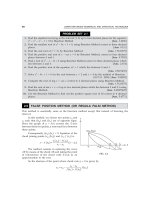
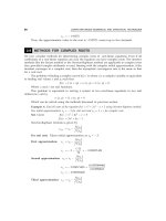
2.5 FALSE POSITION METHOD (OR REGULA FALSI METHOD)
This method is essentially same as the bisection method except that instead of bisecting the
interval.
In this method, we choose two points x
0
and
x
1
such that f(x
0
) and f(x
1
) are of opposite signs.
Since the graph of y = f(x) crosses the X-axis
between these two points, a root must lie in between
these points.
Consequently, f(x
0
) f(x
1
) < 0. Equation of the
chord joining points {x
0

, f(x
0
)} and {x
1
, f (x
1
)} is

()
() ()
()
10
00
10
fx fx
xxx
xx
−
−= −
−
yf
The method consists in replacing the curve
AB by means of the chord AB and taking the point
of intersection of the chord with X-axis as an
approximation to the root.
So the abscissa of the point where chord cuts y = 0 is given by

()
()
()

10
20 0
10
xx
xx fx
fx fx
−
=−
−
Y
X
A{ , ( ) )}
xfx
00
x
0
x
3
x
2
x
3
P( )
x
B
FIG. 2.2
ALGEBRAIC AND TRANSCENDENTAL EQUATION
47
The value of x
2

can also be put in the following form:

()
()
()
()
01 10
2
10
xf x xf x
x
fx fx
−
=
−
In general, the (i + 1)th approximation to the root is given by

() ( )
() ( )
11
1
1
iiii
i
ii
xfx xfx
x
fx fx
−−
+

−
−
=
−
2.5.1 Procedure for the False Position Method to Find the Root of the Equation
f
(
x
) = 0
Step 1: Choose two initial guess values (approximations) x
0
and x
1
(where x
1
> x
0
) such
that f(x
0
).f(x
1
) < 0.
Step 2: Find the next approximation x
2
using the formula

()
()
()

()
01 10
2
10
xf x xf x
x
fx fx
−
=
−
and also evaluate f(x
2
).
Step 3: If f(x
2
) f(x
1
) < 0, then go to the next step. If not, rename x
0
as x
1
and then go to
the next step.
Step 4: Evaluate successive approximations using the formula

() ( )
() ( )
11
1
1

, where = 2, 3, 4,
iiii
i
ii
xfx xfx
xi
fx fx
−−
+
−
−
=
−
But before applying the formula for x
i + 1
, ensure whether f(x
i–1
). f(x
i
) < 0; if not,
rename x
i–2
as x
i–1
and proceed.
Step 5: Stop the evaluation when
1
,
−
−<ε

ii
xx
where
ε
is the prescribed accuracy.
2.5.2 Order (or Rate) of Convergence of False Position Method
The general iterative formula for False Position Method is given by

() ( )
() ( )
11
1
1
iiii
i
ii
xfxxfx
x
fx f x
−−
+
−
−
=
−
(1)
where x
i–1
, x
i

and x
i+1
are successive approximations to the required root of f(x) = 0.
The formula given in (1), can also be written as:

()
()
() ( )
1
1
1
ii i
ii
ii
xx fx
xx
fx fx
−
+
−
−
=−
−
(2)
Let
α
be the actual (true) root of f(x) = 0, i.e., f(
α
) = 0. If e
i–1

, e
i
and e
i+1
are the successive
errors in (i – 1)th, ith

and (i + 1)th iterations respectively, then
e
i–1
= x
i–1
–
α
, e
i
= x
i
–
α
, e
i + 1
= x
i + 1
–
α
or x
i–1
= α + e
i–1

, x
i
=
α
+ e
i
, x
i+1
=
α
+ e
i+1
48
COMPUTER BASED NUMERICAL AND STATISTICAL TECHNIQUES
Using these in (2), we obtain

()()
()( )
1
1
1
ii i
ii
ii
ee f e
ee
fefe
−
+
−

−α+
α+ =α+ −
α+ − α+
or
()
()
()
()
1
1
1
ii i
ii
ii
ee f e
ee
fefe
−
+
−
−α+
=−
α+ − α+
(3)
Expanding f(
α
+ e
i
) and f(α + e
i –1

) in Taylor’s series around
α
, we have

()
() () ()
() () () () () ()
1
2
1
1
22
1

2

22
i
ii
ii i
ii
ii
e
ee f ef f
ee
ee
fef f fef f
−
−
+

−

′′′
−α+α+α+



=−
 
′′′ ′′
α+ α+ α+ − α+ ′α+ α+
 
 
 
i.e.,
()
() () ()
()
() ()
−
+
−
−

′′′
−α+α+α



=−



−
′′′
−α+ α





2
1
1
22
1
1

2


2
i
ii i
ii
ii
ii
e
ee f ef f
ee
ee

ee f f
, [on ignoring the higher order terms]
i.e.
() () ()
() ()
+
−

′′′
α+ α+ α


==
+


′′
α+ α




2
1
1
2

'
2
i

i
ii
ii
e
fef f
ee
ee
ff
i.e.
() ()
()
()
−

′′′
α+ α


−
+


′′′
α+ α




2
+ 1

1
2
=
2
i
i
ii
ii
e
ef f
ee
ee
ff
[since f(
α
) = 0]
i.e.
()
()
()
()
2
1
1
2
1
2
i
i
ii

ii
f
e
e
f
ee
fee
f
+
−
′′
α
+

′
α

=−
′′

α+

+


′
α


,

[on dividing numerator and denominator by f ′(
α
)
i.e.
()
()
()
()
1
2
1
1
1
22
iii
iii
ff
eee
eee
ff
−
−
+

′′ ′′

αα
+

=− + +




′′
αα




i.e.
()
()
()
()
2
1
1
1
22
ii
i
iii
ff
eee
eee
ff
−
+
′′ ′′


αα
+

=− + −



′′
αα



ALGEBRAIC AND TRANSCENDENTAL EQUATION
49
i.e.,
()
()
()
()
2
22
11
1
()
() ()
22()4
ii i i i i i
ii
ff
f

ee e e e e e
ee
ff f
−−
+

′′ ′′
′′  
αα
α
++


=− + −

′′ ′
αα α




i.e.,
()
()
()
+
′′
α
=− +
′

α
1
2
1
0
2
iii i
f
eee e
f
If e
i–1
and e
i
are very small, then ignoring 0(e
2
i
), we get

()
()
11
2
iii
f
eee
f
+−
′′
α

=
′
α
(4)
which can be written as
e
i + 1
= e
i
e
i–1
M, where M =
()
()
2
f
f
′′
α
′
α
and would be a constant (5)
In order to find the order of convergence, it is necessary to find a formula of the type
e
i + 1
= Ae
k
i
with an appropriate value of k. (6)
With the help of (6), we can write

e
i
= Ae
1
k
i−
or e
i–1
= (e
i
/A)
1/k
Now, substituting the value of e
i+1
and e
i–1
in (5), we get
Ae
k
i
= e
i
.
1/
.
k
i
e
M
A




or e
k
i
= MA
–(1 + 1/k)
.e
i
(1+1/k)
(7)
Comparing the powers of e
i
on both sides of (7), we get
k = 1 + (1/k)
or k
2
– k – 1 = 0 (8)
From (8), taking only the positive root, we get k = 1.618
By putting this value of k in (6), we have

i+1
1.618
1
1.618
or
ii
i
e

eAe A
e
+
==
Comparing this with
1
lim
i
k
i
i
e
A
e
+
→∞

≤



, we see that order (or rate) of convergence of false
position method is 1.618.
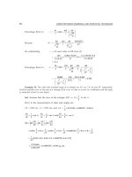
Example 1. Find a real root of the equation f(x) = x
3
– 2x – 5 = 0 by the method of false position
up to three places of decimal.
Sol. Given that f(x)= x
3
– 2x – 5 = 0

So that f(2) = (2)
3
– 2(2) – 5 = – 1
50
COMPUTER BASED NUMERICAL AND STATISTICAL TECHNIQUES
and f(3) = (3)
3
– 2(3) – 5 = 16
Therefore, a root lies between 2 and 3.
First approximation: Therefore taking x
0
= 2, x
1
= 3, f(x
0
) = – 1, f(x
1
)= 16, then by Regula-
Falsi method, we get

()
()
()
10
20 0
10
xx
xx fx
fx fx
−

=−
−
()
32 1
2 1 2 2.0588
16 1 17
−
=− −=+ =
+
Now, f(x
2
)= f(2.0588)
= (2.0588)
3
– 2 (2.0588) – 5 = – 0.3911
Therefore, root lies between 2.0588 and 3.
Second approximation: Now, taking x
0
= 2.0588, x
1
= 3, f(x
0
) = – 0.3911, f(x
1
) = 16, then by
Regula-Falsi method, we get

()
()
()

10
30 0
10
xx
xx fx
fx fx
−
=−
−
= 2.0588 –
3 2.0588
16 0.3911
−
+
(– 0.3911) = 2.0588 + 0.0225 = 2.0813
Now, f(x
3
)= f (2.0813)
= (2.0813)
3
– 2(2.0813) – 5 = – 0.1468
Therefore, root lies between 2.0813 and 3.
Third approximation: Taking x
0
= 2.0813 and x
1
= 3, f(x
0
) = – 0.1468, f(x
1

) = 16. Then by
Regula-Falsi method, we get

()
()
()
10
40 0
10
xx
xx fx
fx fx
−
=−
−
= 2.0813 –
3 2.0813
16 0.1468
−
+
(– 0.1468) = 2.0813 + 0.0084 = 2.0897
Now, f(x
4
)= f(2.0897)
= (2.0897)
3
– 2 (2.0897) – 5
= 9.1254 – 9.1794 = – 0.054
Therefore, root lies between 2.0897 and 3.
Fourth approximation: Now, taking x

0
= 2.0897, x
1
= 3, f (x
0
) = – 0.054, f (x
1
) = 16, then by
Regula-Falsi method, we get

()
()
()
10
50 0
10
xx
xx fx
fx fx
−
=−
−
= 2.0897 –
()
3 2.0897
0.054
16 0.054
−
−
+

= 2.0897 + 0.0031 = 2.0928
ALGEBRAIC AND TRANSCENDENTAL EQUATION
51
Now, f(x
5
)= f(2.0928)
= (2.0928)
3
– 2(2.0928) – 5
= 9.1661 – 9.1856 = – 0.0195
Therefore, root lies between 2.0928 and 3.
Fifth approximation: Now, taking x
0
= 2.0928, x
1
= 3, f(x
0
) = – 0.0195, f(x
1
) = 16, then we
get

()
()
()
10
60 0
10
xx
xx fx

fx fx
−
=−
−
= 2.0928 –
()
3 2.0928
0.0195
16 0.0195
−
−
+
= 2.0928 + 0.0011 = 2.0939
Now, f(x
6
)= f(2.0939)
= (2.0939)
3
– 2 (2.0939) – 5
= 9.1805 – 9.1879 = – 0.0074
Thus the root lies between 2.0939 and 3.
Sixth approximation: Now, taking x
0
= 2.0939, x
1
= 3, f(x
0
) = – 0.0074, f(x
1
) = 16, then we

get

()
()
()
10
70 0
10
xx
xx fx
fx fx
−
=−
−
= 2.0939 –
()
32.0939
0.0074
16 0.0074
−
−
+
= 2.0939 + 0.00042 = 2.0943
Now, f(x
7
)= f(2.0943)
= (2.0943)
3
– 2(2.0943) – 5
= 9.1858 – 9.1886 = – 0.0028

Therefore, root lies between 2.0943 and 3.
Seventh approximation: Taking x
0
= 2.0943, x
1
= 3, f(x
0
) = – 0.0028, f(x
1
) = 16, then by Falsi
position method, we get

()
()
()
10
80 0
10
xx
xx fx
fx fx
−
=−
−
= 2.0943 –
()
32.0943
0.0028
16 0.0028
−

−
+
= 2.0943 + 0.00016 = 2.0945
Hence, the root is 2.094 correct to three decimal places.
Example 2. Find the real root of the equation f(x) = x
3
– 9x + 1 = 0 by Regula-Falsi method.
Sol. Let f(x)= x
3
– 9x + 1 = 0 (1)
So that f(2) = (2)
3
– 9(2) + 1 = – 9
f(3) = (3)
3
– 9(3) + 1 = 1
52
COMPUTER BASED NUMERICAL AND STATISTICAL TECHNIQUES
Since f(2) and f(3) are of opposite signs, therefore the root lies between 2 and 3, so taking
x
0
= 2, x
1
= 3, f(x
0
) = – 9, f(x
1
) = 1, then by Regula-Falsi method, we get
First approximation:
()

()
()
10
20 0
10
xx
xx fx
fx fx
−
=−
−
()
32 9
2922.9
19 10
−
=− ×−=+ =
+
Now, f(x
2
)= f(2.9)
= (2.9)
3
– 9 (2.9) + 1
= 24.389 – 25.1 = – 0.711
Second approximation: The root lies between 2.9 and 3. Therefore, taking x
0
= 2.9, x
1
= 3,

f(x
0
) = – 0.711, f(x
1
) = 1. Then

()
()
()
10
30 0
10
xx
xx fx
fx fx
−
=−
−
= 2.9 –
()
32.9
0.711
1 0.711
−
−
+
= 2.9 + 0.0416 = 2.9416
Now, f(x
3
)= f(2.9416)

= (2.9416)
3
– 9(2.9416) + 1
= 25.4537 – 25.4744 = – 0.0207
Third approximation: The root lies between 2.9416 and 3. Therefore, taking x
0
= 2.9416,
x
1
= 3, f(x
0
) = – 0.0207, f(x
1
) = 1. Then we get

()
()
()
10
40 0
10
xx
xx fx
fx fx
−
=−
−
= 2.9416 –
()
32.9416

0.0207
10.0207
−
−
+
= 2.9416 + 0.0012 = 2.9428
Now, f(x
4
)= f (2.9428)
= (2.9428)
3
– 9(2.9428) + 1
= 25.4849 – 25. 4852 = – 0.0003
Fourth approximation: The root lies between 2.9428 and 3. Therefore, taking
x
0
= 2.9428, x
1
= 3, f (x
0
) = – 0.0003, f (x
1
) = 1. Then by False Position method, we have

()
()
()
10
50 0
10

xx
xx fx
fx fx
−
=−
−
= 2.9428 –
()
3 2.9428
0.0003
1 0.0003
−
−
+
= 2.9428 + 0.000017 = 2.942817
Hence, the root is 2.9428 correct to four places of decimal.
ALGEBRAIC AND TRANSCENDENTAL EQUATION
53
Example 3. Using the method of False Position, find the root of equation x
6
– x
4
– x
3
–1 = 0 up
to four decimal places.
Sol. Let f(x) = x
6
– x
4

– x
3
– 1
f(1.4) = (1.4)
6
– (1.4)
4
– (1.4)
3
– 1 = – 0.056
f(1.41) = (1.41)
6
– (1.41)
4
– (1.41)
3
– 1 = 0.102
Hence the root lies between 1.4 and 1.41.
Using the method of False Position,

()
()
()
10
20 0
10
xx
xx fx
fx fx
−

=−
−
= 1.4 –
()
1.41 1.4
0.056
0.102 0.056
−
−
+
= 1.4 +
()
0.01
0.056 1.4035
0.158

=


Now, f (1.4035) = (1.4035)
6
– (1.4035)
4
– (1.4035)
3
– 1
f (x
2
) = – 0.0016 (–ve)
Hence the root lies between 1.4035 and 1.41.

Using the method of False Position,

() ()
()
12
32 2
12
xx
xx fx
fx fx
−
=−
−
= 1.4035 –
−
−
+
1.41 1.4035
( 0.0016)
0.102 0.0016
= 1.4035 +
()
0.0065
0.0016 1.4036
0.1036

=


Now, f(1.4036) = (1.4036)

6
– (1.4036)
4
– (1.4036)
3
– 1
f(x
3
) = – 0.00003 (–ve)
Hence the root lies between 1.4036 and 1.41.
Using the method of False Position,

()
()
()
13
43 3
13
xx
xx fx
fx fx
−
=−
−
= 1.4036 –
()
1.41 1.4036
0.00003
0.102 0.00003
−

−
+
= 1.4036 +
()
0.0064
0.00003 1.4036
0.10203

=


Since, x
3
and x
4
are approximately the same upto four places of decimal, hence the required
root of the given equation is 1.4036.
54
COMPUTER BASED NUMERICAL AND STATISTICAL TECHNIQUES
Example 4. Find a real root of the equation f(x) = x
3
– x
2
– 2 = 0 by Regula-Falsi method.
Sol. Let f(x)= x
3
– x
2
– 2 = 0
Then, f(0) = – 2, f(1) = – 2 and f(2) = 2

Thus, the root lies between 1 and 2.
First approximation: Taking
1
00
1, 2, ( )
2
x
xfx== =−
and
1
()
fx
= 2. Then by Regula-Falsi
method, an approximation to the root is given by

10
20 0
1) 0
()
(()
xx
xx fx
fx fx
−
=−
−
21 1
1(2)11.5
22 2
−

=− − =+ =
+
Now,
2
() (1.5)
fx f=
= (1.5)
3
– (1.5)
2
– 2
= 3.375 – 4.25 = – 0.875
Thus, the root lies between 1.5 and 2.
Second approximation: Taking
01 0
1.5, 2, ( ) 0.875
xxfx== =−
and
1
()2.
fx =
Then the next
approximation to the root is given by

10
30 0
1) 0
()
(()
xx

xx fx
fx fx
−
=−
−
= 1.5 –
()
21.5
0.875
20.875
−
−
+
= 1.5 + 0.1522 = 1.6522
Now, f(x
3
)= f(1.6522)
= (1.6522)
3
– (1.6522)
2
– 2
= 4.5101 – 4.7298 = – 0.2197
Thus, the root lies between 1.6522 and 2.
Third approximation: Taking x
0
= 1.6522, x
1
= 2, f(x
0

) = – 0.2197 and f(x
1
) = 2. Then the next
appoximation to the root is given by

10
40 0
1) 0
()
(()
xx
xx fx
fx fx
−
=−
−
= 1.6522 –
()
2 1.6522
0.2197
2 0.2197
−
−
+
= 1.6522 + 0.0344 = 1.6866
Now, f(x
4
)= f(1.6866)
= (1.6866)
3

– (1.6866)
2
– 2
= 4.7977 – 4.8446 = – 0.0469
Thus, the root lies between 1.6866 and 2.
ALGEBRAIC AND TRANSCENDENTAL EQUATION
55
Fourth approximation: Taking x
0
= 1.6866, x
1
= 2, f (x
0
) = – 0.046 and f (x
1
) = 2. Then the
root is given by

10
50 0
1) 0
()
(()
xx
xx fx
fx fx
−
=−
−
= 1.6866 –

()
1.6866
0.0469
2 0.0469
−
−
+
= 1.6866 + 0.0072 = 1.6938
Now, f(x
5
)= f(1.6938)
= (1.6938)
3
– (1.6938)
2
– 2
= 4.8594 – 4.8690 = – 0.0096
Thus, the root lies between 1.6938 and 2.
Fifth approximation: Taking x
0
= 1.6938, x
1
= 2, f(x
0
) = – 0.0096 and f(x
1
) = 2. Then the next
approximation to the root is given by

10

60 0
1) 0
()
(()
xx
xx fx
fx fx
−
=−
−
= 1.6938 –
()
2 1.6938
0.0096
2 0.0096
−
−
+
= 1.6938 + 0.0015 = 1.6953
Now, f(x
6
)= f(1.6953)
= (1.6953)
3
– (1.6953)
2
– 2
= 4.8724 – 4.8740 = – 0.0016
Therefore, the root lies between 1.6953 and 2.
Sixth approximation: Taking x

0
= 1.6953, x
1
= 2, f(x
0
) = – 0.0016 and f(x
1
) = 2. Then the next
approximation to the root is

10
70 0
1) 0
()
(()
xx
xx fx
fx fx
−
=−
−
= 1.6953 –
()
2 1.6953
0.0016
2 0.0016
−
−
+
= 1.6953 + 0.0002 = 1.6955

Hence, the root is 1.695 correct to three places of decimal.
Example 5. Find a real root of the equation f(x) = xe
x
– 3 = 0, using Regula-Falsi method correct
to three decimal places.
Sol. We have f(x)= xe
x
– 3 = 0
Then f(1) = 1e
1
– 3 = – 0.2817
and f(1.5) = (1.5)e
(1.5)
– 3 = 3.7225.
∴
The root lies between 1 and 1.5. Therefore, taking x
0
= 1, x
1
= 1.5, f(x
0
) = – 0.2817 and
f(x
1
) = 3.7225. The first approximation to the root is