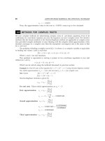
A textbook of Computer Based Numerical and Statiscal Techniques part 12 pdf

96
COMPUTER BASED NUMERICAL AND STATISTICAL TECHNIQUES
Now to obtain the values of b
i
and C
i
we use the following procedure:
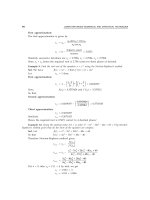
1 6 18 24 16
1.5 1.5 6.75 15.375 6.1875
1 1 4.5 10.25
1 4.5 10.25 4.125 0.4375
1.5 1.5 4.5 7.125 9
1134.75
1 3 4.75 6 3.8125
−−
−−
−−−
−−−
−
−−−
−
Here from the table b
3
= –4.125, b
4
= –0.4375, C
1
= –3, C
2
= 4.75, C
3

= 6 therefore after
substituting the values of b
i
and C
i
in equations (1) and (2) we get
∆p = –
1.3125 19.59
4
22.56 3(10.12
5)
+
+
∆p = –0.3949
∆q = –
( 39.687
5)
( 52.935
)
−
∆q = 0.74974
Therefore the first approximation are given by
p
1
= p
0
+ ∆p = –1.5 + (–0.3949) = –1.8949
q
1
= q

0
+ ∆q = 1 + 0.74974 = 1.74974
Second approximation: Using p
1
= –1.8949 and q
1
= 1.74974 for second approximation, then
p
2
= p
1
+ ∆p and q
2
= q
1
+ ∆q.
Now to obtain the values of b
i
and C
i
we use the following procedure:
−−
−−
−−−
−−−
−
−−−
−
1 6 18 24 16
1.8949 1.8949 7.7787 16.0526 1.4487

1.74974 1.74974 7.1828 14.8229
1 4.1051 8.4715 0.7645 0.2716
1.8949 1.8949 4.188 4.801 15.4044
1.74974 1.74974 3.8673 4.433
1 2.2102 2.5336 7.9038 10.6996
i
i
i
a
b
C
After substituting the values of b
i
and C
i
in equations (1) and (2) we get
∆p =
2.53722752
25.57781
ALGEBRAIC AND TRANSCENDENTAL EQUATION
97
∆p = –0.09919
∆q =
( 5.9387
9)
25.5778
1
−
∆q = 0.23218
Therefore the second approximations are given by

p
2
= p
1
+ ∆p = –1.99409
q
2
= q
1
+ ∆q = 1.98192
Third approximation: Using p
2
= –1.99409 and q
2
= 1.98192 for third approximation, then
p
3
= p
2
+ ∆p and q
3
= q
2
+ ∆q.
Now to obtain the values of b
i
and C
i
we use the following procedure:
−−

−−
−−−
−−−
−
−−−
−
1 6 18 24 16
1.99409 1.99409 7.988 16.0124 0.096
2
1.98192 1.98192 7.9394 15.91
46
1 4.0059 8.0299 0.048226 0.010
82
1.99409 1.99409 4.01173 4.06046 15.95
2
1.98192 1.98192 3.9873 4.035
7
1 2.0118 0.03625 7.9995 11.9
i
i
i
a
b
C
05
5
After substituting the values of b
i
and C
i

in equations (1) and (2) we get
p
∆
=
0.1199
7
20.336
7
p
∆
= – 0.005899
q
∆
= –
()
0.3660
7
20.3367
−
q
∆
= 0.01800
Therefore the third approximation are given by
p
3
= p
2
+ ∆p = –1.9882
q
3

= q
2
+ ∆q = 1.9999
Thus, we obtain p = –1.9882 and q = 1.9999. Hence quadratic factor of the given equation
is x
2
– 1.9882x + 1.9999 = 0. Now if root of the quadratic factor is
i
α± β
, then
2α = 1.9882 ⇒ α = 0.9941, α
2
+ β
2
= 1.9999 ⇒ β = 1.0058
Hence a pair of roots is 0.9941
±
1.0058i
Other roots can be obtained by using default polynomial.
Default polynomial is given by b
0
x
2
+ b
1
x + b
2
= 0, where b
i
are given by the same procedure,

when p and q are of required accuracy.
98
COMPUTER BASED NUMERICAL AND STATISTICAL TECHNIQUES
1
1 6 18 24 16
1.9882 1.9882 7.97626 15.95299 0.047343
1.9999 1.9999 8.023198 16.04687
1 4.0118 8.02384 0.023812 0.094213
i
a
b
−−
−−
−−−
−−−
Thus b
0
= 1, b
1
= –4.0118, b
2
= 8.02384 and thus the polynomial becomes 1x
2
– 4.0118x
+ 8.02384 = 0, whose roots are γ = 2.0059, δ = 2.00005
Hence the pair of roots is
2.0059 2.0000
5i
±
Example 10. Solve x

4
– 5x
3
+ 20x
2
– 40x + 60 = 0 given that all the roots are complex, by using
Lin-Bairstow method. Take the values as p
0
= –4, q
0
= 8.
Sol. Let the quadratic factor of the equation be x
2
+ px + q. Using Bairstow’s method we find
the values of p and q:
First approximation: Let p
0
and q
0
be the initial approximations, then the first approximation
can be obtained p
1
= p
0
+ ∆p and q
1
= q
0
+ ∆q. Because given equation is of the degree four then
∆p = –

41 32
2
2133
()
−
−−
bC bC
CCCb
(1)
∆q = –
33 3 4
2
2
2133
()
(
)
bC b bC
CCCb
−−
−−
(2)
Now to obtain the values of b
i
and C
i
we use the following procedure:
1 5 20 40 60
444320
88864

118 0 4
4 4 12 48 96
8 8 24 96
1 3 12 24 4
i
i
i
a
b
C
−−
−
−−−
−−
−−−−
−
Here from the table b
3
= 0, b
4
= –4, C
1
= 3, C
2
= 12, C
3
= 24 therefore after substituting the
values of b
i
and C

i
in equations (1) and (2), we get
∆p = –
2
(4) 3 0(12
)
(12) 3 (24
0)
−×−×
−× −
∆p = 0.166666
∆q = –
2
0(240) (4)1
2
( 12) 3 ( 24 0)
×−−−×
−× −
∆q = –0.666666
ALGEBRAIC AND TRANSCENDENTAL EQUATION
99
Therefore the first approximation are given by
p
1
= p
0
+ ∆p = –4 + 0.166666 = –3.833334
q
1
= q

0
+ ∆q = 8 – 0.666666 = 7.333334
Second approximation: Using p
1
= –3.833334 and q
1
= 7.333334 for second approximation,
then p
2
= p
1
+ ∆p and q
2
= q
1
+ ∆q.
Now to obtain the values of b
i
and C
i
we use the following procedure:
1 5 20 40 60
3.833334 3.833334 4.472220 31.412048 0.124203
7.333334 7.333334 8.555551 60.092609
1 1.166666 8.194446 0.032401 0.216812
3.833334 3.8333334 10.222229 42.486147 87.7763681
7.333334 7.333334 19.5555
i
i
a

b
−−
−−
−−−
−−−
−−−
67 81.277841
1 2.666668 11.083341 22.898179 6.2817151
i
C
−
After substituting the values of b
i
and C
i
in equations (1) and (2), we get
∆p = –0.015192
∆q = –0.026908
Therefore the second approximation are given by
p
2
= p
1
+ ∆p = –3.833334 – 0.015192 = –3.848526
q
2
= q
1
+ ∆q = 7.333334 – 0.026908 = 7.306426
Third approximation: Using p

2
= – 3.848526 and q
2
= 7.306426 for third approximation,
then p
3
= p
2
+ ∆p and q
3
= q
2
+ ∆q.
Now to obtain the values of b
i
and C
i
we use the following procedure
1 5 20 40 60
3.848526 3.848526 4.431477 31.796895 0.808398
7.306426 7.306426 8.413159 60.366400
1 1.151474 8.262097 0.210054 0.441998
3.848526 3.848526 10.379674 43.624369 92.859594
7.306426 7.306426 19.705810 82
i
i
a
b
−−
−

−−−
−
−−−−
.820859
1 2.697052 11.335345 24.128613 10.480733
i
C
After substituting the values of b
i
and C
i
in equations (1) and (2), we get
∆p = 0.018582
∆q = – 0.0002186
100
COMPUTER BASED NUMERICAL AND STATISTICAL TECHNIQUES
Therefore the third approximation are given by
p
3
= p
2
+ ∆p= –3.848526 + 0.018582 = – 3.829944
q
3
= q
2
+ ∆q= 7.306426 – 0.000218 = 7.306208
Thus, we obtain p = – 3.83 and q = 7.3062. Hence quadratic factor of the given equation is
x
2

– 3.83x + 7.3062. Now if root of the quadratic factor is α ± iβ
2
, then
2α = 3.83 ⇒ α = 1.915, α
2
+ β
2
= 7.3062 ⇒ β = 1.9081
Hence a pair of roots is 1.915 ± 1.908li
Other roots can be obtained by using default polynomial.
Default polynomial is given by b
0
x
2
+ b
1
x + b
2
= 0, where b
i
are given by the same procedure,
when p and q are of required accuracy.
−−
−
−−−
−
1
1 5 20 40 60
3.829944 8.829944 4.481248 31.453583 0.00863
6

7.306208 7.306208 8.548672 60.0025
54
1 1.170056 8.212544 0.002255 0.006081
85
i
a
b
Thus b
0
= 1, b
1
= – 1.17, b
2
= 8.2125 and thus the polynomial becomes 1x
2
– 1.17x +
8.2125 = 0, whose roots are γ = 0.585, δ = 2.8054.
Hence the pair of roots is 0.585 ± 2.8054i.
2.12 QUOTIENT DIFFERENCE METHOD
This is a general method to obtain the approximate roots of the polynomial equations. The procedure
is quite general and is illustrated here with a cubic polynomial. Let the given cubic equation be
f(x) = a
0
x
3

+ a
1
x
2

+ a
2
x + a
3
= 0 (1)
and let x
1
, x
2
and x
3
be its root such that 0 <
123
xxx<<
The roots can be obtained, directly by considering the transformed equation
a
3
x
3
+ a
2
x
2
+ a
1
x + a
0
= 0 (2)
Whose roots are the reciprocals of those of (1).
We then have

32
3210
0
1
i
i
i
x
ax ax ax a
∞
=
=α
+++
∑
So that (a
3
x
3
+ a
2
x
2
+

a
1
x

+ a
0

) (α
0
+ α
1
x + α
2
x
2
+ )=1 (3)
Comparing the coefficients of like powers of x on both sides of (3), we get
α
0
=
0
1
a
, α
1
= –
1
2
0
a
a
, α
2
=
2
2
1

2
3
0
0
a
a
a
a
−
+
Hence, q
1
(1)
=
1
0
α
α
= –
1
0
a
a
ALGEBRAIC AND TRANSCENDENTAL EQUATION
101
q
1
(2)
=
2

1
α
α
=
−
2
20
1
01
aa
a
aa
And so, ∆
1
(1)
= q
1
(2)
– q
(1)

=
2
1
a
a
, ∆
2
(0)
=

3
2
a
a
In general, ∆
m
(m)
=
1
m
m
a
a
+
, m = 1, 2, 3, (n – 1)
q
m
(1–m)
= 0, m = 2, 3, , n
That is q
1
(0)
, q
2

(–1)
, q
3

(–2)

, , top q’s are 0.
We also set ∆
0
(k)
=∆
n
(k)
= 0, for all k. [i.e., first and last columns of Q-d table are zero].
The Quotient Difference table for a Cubic Equation
q
1
(0)
q
2
(–1)
q
3
(–2)
∆
0
(1)
∆
1
(0)
∆
2
(–1)
∆
3
(–2)

q
1
(1)
q
2
(0)
q
3
(–1)
∆
0
(2)
∆
1
(1)
∆
2
(0)
∆
3
(–1)
q
1
(2)
q
2
(1)
q
3
(0)

∆
0
(3)
∆
1
(2)
∆
2
(1)
∆
3
(0)
Remarks:
(1) If an ∆ element is at the top of the rhombus, then the product of one pair is equal to that
of the other pair. For example, in the rhombus
∆
1
(1)
q
1
(2)
q
2
(1)
We have ∆
1
(1)
.q
2
(1)

= ∆
1
(2)
.q
1
(2)
∆
1
(2)
From which ∆
1
(2)
can be computed since the other quantities are known.
(2) If a q-element is at the top, then the sum of one pair is equal to that of the other pair. For
example, in the rhombus
q
2
(0)
∆
1
(1)
∆
2
(0)
We have q
2
(0)
+ ∆
2
(0)

= q
2
(1)
+ ∆
1
(1)
q
2
(1)
From which q
2
(1)
can be computed when q
2
(0)
, ∆
1
(1)
, ∆
2
(0)
are known.
As the building up of table proceeds, the quantities q
1
(i)
, q
2
(i)
, q
3

(i)
tend to roots of cubic
equations. The disadvantage of this method is that additional computation is also necessary. This
method can be applied to find the complex roots and multiple roots of polynomials and also for
determining the Eigen values of a matrix.
An important feature of the method is that it gives approximate values of all the roots
simultaneously and this fact enables one to use this method to obtain the first approximations of
all roots and then apply a rapidly convergent method such as the generalized Newton method
to obtain the roots to the desired accuracy.
102
COMPUTER BASED NUMERICAL AND STATISTICAL TECHNIQUES
Example 11. Solve the following equation by using quotient-difference method x
3
– 6x
2
+
11x – 6 = 0.
Sol. To obtain the roots directly, we consider the transformed equation
–6x
3
+ 11x
2
– 6x + 1 = 0
Here a
3
= – 6, a
2
= 11, a
1
= – 6 and a

0
= 1.
Therefore, we have q
1
(1)
= –
1
0
a
a
= 6
q
1
(2)
= –
2
20
1
01
aa
a
aa
−
=
11 3
6
6
−
−
= 4.167

∆
1
(1)
= q
1
(2)
– q
1
(1)
=
2
1
a
a
= – 1.833
Also q
2
(0)
= 0, q
3
(–1)
= 0 and ∆
2
(0)
=
3
2
a
a
= `

6
11
= – 0.5454
First two rows containing starting values of
() ()
() () () ( )
10
(1)
12 3
21 0 1
01 2 3
60 0
0 1.833 0.5454 0
qq q
−
−
∆∆ ∆ ∆
−−
The succeeding rows can be constructed as below:
0112233
600
0 1.833 0.545 0
4.167 1.288 0.5454
0 0.5666 0.2310 0
3.600 1.624 0.7764
0 0.2556 0.1105 0
3.344 1.770 0.8869
0 0.1353 0.0553 0
3.209 1.8550 0.9422
0 0.0782 0.0281 0

3.131 1.9051 0.9703
0 0.0476 0.0143 0
3.083 1.
qqq∆∆ ∆ ∆
−−
−−
−−
−−
−−
−−
9384 0.9846
0 0.0299 0.0073 0
3.053 1.961 0.9919
0 0.0192 0.0037 0
3.0338 1.976 0.9956
−−
−−
It is evident that q
1
, q
2
, q
3
are gradually converging to the roots 3, 2 and 1 respectively.
ALGEBRAIC AND TRANSCENDENTAL EQUATION
103
PROBLEM SET 2.5
1. Use Secant method to determine the root of the equation cos x – xe
x
= 0.

[Ans. 0.5177573637]
2. Using Secant method, find the root of x–e
–x
= 0 correct to three decimal places by taking
x
0
= 1 and x
1
= 1.5. [Ans. 1.114]
3. Apply Muller’s method to obtain the root of the equation cos x – xe
x
= 0 which lies between
0 and 1. [Ans. 0.518]
4. Solve by Muller’s method x
3
+ 2x
2
+ 10x –20 = 0 by taking x = 0, x = 1, x = 2 as initial
approximation. [Ans. 1.368808108]
5. Find a quadratic factor of the polynomial x
4
+ 5x
3
+ 3x
2
– 5x – 9 = 0. Starting with p
0
= 3,
q
0

= – 5 by using Bairstow’s Method. [Ans. x
2
+ 2.90255x – 4.91759]
6. Solve the equation x
4
– 8x
3
+ 39x
2
– 62x + 50 = 0. Starting with p = 0, q = 0.
7. Find the real roots of the equation x
3
– 7x
2
+ 10x – 2 = 0 by using Quotient difference
method. [Ans. 5.12487, 1.63668, 0.23845]
8. Solve the following equation x
3
– 8x
2
+ 17x – 10 = 0 by using Quotient difference method.
[Ans. 5, 2.001, 0.9995]
9. Find all the roots of the equation x
3
– 5x
2
– 17x + 20 = 0 by using Quotient difference
method. [Ans. 7.018, –2.974, 0.958]
GGG
CHAPTER 3

Calculus of Finite Differences
3.1. INTRODUCTION
Finite differences: The calculus of finite differences deals with the changes that take place in the
value of the dependent variable due to finite changes in the independent variable from this we
study the relations that exist between the values, which can be assumed by function, whenever
the independent variable changes by finite jumps whether equal or unequal.
The study of finite difference calculus has become very important due to its wide variety
of application in routine life. It has been originated by Sir Issac Newton. It has been of great use
for Mathematicians as well as Computer Scientists for solution of the Scientific, business and
engineering problems. There it helps in reducing complex mathematical expressions like
trigonometric functions in terms of simple arithmetic operations.
3.2 FINITE DIFFERENCES
Numerical methods are very important tools to provide practical methods for calculating the
solution of problems to applied mathematics for a desired degree of accuracy.
If f is a function from x into y for a ≤ x ≤ b such that y = f(x), this means that one or more
values of y = f(x) exist corresponding to every value of x in the given range. However if the
function f is not known, the value of y can be obtained, when a set of values of x is given. The
method to find out such values is based on principle of finite differences provided the function
is continuous.
3.3 ARGUMENT AND ENTRY
If y = f(x) be a function assumes the values f(a), f(a + h), f(a + 2h), corresponding to the values
of x then each value of x is called argument and its corresponding values of y is called entry.
3.4 DIFFERENCES
Let y = f(x) be a function tabulated for the equally spaced values or argument a = x
0
, x
0
+ h, x
0
+ 2h, , x

0
+ 2h, x
0
+ nh, where h is the increment given to the independent variable of
function y = f(x). To determine the values of function y = f(x) for given intermediate or argument
values of x, three types of differences are useful:
104
CALCULUS OF FINITE DIFFERENCES
105
3.4.1 Forward or Leading Differences
If we subtract from each value of y except y
0
, the previous value of y, we have
y
1
– y
0
, y
2
– y
1
, y
3
– y
2
, , y
n
– y
n–1
. These differences are called the first forward differences

of y and is denoted by ∆y. The symbol ∆ denotes the forward difference operator. That is,
∆y
0
= y
1
– y
0
∆y
1
= y
2
– y
1
∆y
2
= y
3
– y
2
.
.
.
∆y
n
= y
n+1
– y
n
Also it can be written as,
∆f(x)= f(x+h) – f(x)

where h is the interval of differencing.
Similarly for second and higher order differences,
∆
2
y
0
= ∆y
1

– ∆y
0
∆
2
y
1
= ∆y
2

– ∆y
1

∆
2
y
n–1
= ∆y
n

– ∆y
n–1

or ∆
3
y
0
= ∆
2
y
1

– ∆
2
y
0
∆
3
y
1
= ∆
2
y
2

– ∆
2
y
1

∆
3
y

n–1
= ∆
2
y
n

– ∆
2
y
n–1
In general, nth forward difference are given by
∆
n
y
r
= ∆
n–1
y
r–1

– ∆
n–1
y
r,
or
∆
n
f(x)= ∆
n–1
f(x + h)

– ∆
n–1
f(x)
Forward Difference Table:
234
00
0
2
01 0
3
10
24
02 1 0
3
21
2
03 2
3
04
2
3
4
xy
xy
y
xhy y
yy
xhy y y
yy

xhy y
y
xhy
∆∆ ∆ ∆
∆
+∆
∆∆
+∆∆
∆∆
+∆
∆
+
where x
0
+ h = x
1
, x
0
+ 2h = x
2
, , x
0
+ nh = x
n