A textbook of Computer Based Numerical and Statiscal Techniques part 13 doc

106
COMPUTER BASED NUMERICAL AND STATISTICAL TECHNIQUES
Example 1. Construct a forward difference table for the following values:
0 5 10 15 20 25
()71114182432
x
fx
Sol. Forward difference table for given data is:
∆∆∆∆∆
−
−
−
2345
07
4
511 1
32
10 14 1 1
410
15 18 2 1
60
20 24 2
8
25 32
xyyyyyy
Example 2. If y = x
3
+ x
2
– 2x + 1, calculate values of y for x = 0, 1, 2, 3, 4, 5 and form the
difference table. Also find the value of y at x = 6 by extending the table and verify that the same value

is obtained by substitution.
Sol. For x = 0, 1, 2, 3, 4, 5, we get the values of y are 1, 1, 9, 31, 73, 141. Therefore, difference
table for these data is as:
23
01
0
11 8
86
29 14
22 6
331 20
42 6
473 26
68 6
5141 32
100
6241
xyy y y∆∆ ∆
Because third differences are zero therefore
∆
3
y
3
= 6 ⇒∆
2
y
4
– ∆
2
y

3
= 6
⇒∆
2
y
4
–26 = 6 ⇒∆
2
y
4
= 32
Now, ∆
2
y
4
= 32 ⇒∆y
5
– ∆y
4
= 32
CALCULUS OF FINITE DIFFERENCES
107
⇒∆y
5
– 68 = 32 ⇒∆y
5
= 100
Further, ∆y
5
= 100 ⇒ y

6
– y
5
= 100
⇒ y
6
– 141 = 100 ⇒ y
6
= 241
Verification: For given function x
3
+ x
2
– 2x + 1, at x = 6, y(6) = (6)
3
+ (6)
2
– 2(6) + 1 = 241
Hence Verified.
Example 3. Given f(0) = 3, f(1) = 12, f(2) = 81, f(3) = 200, f(4) = 100 and f(5) = 8. From the
difference table and find ∆
5
f(0).
Sol. The difference table for given data is as follows:
2345
() () () () () ()
03
9
112 60
69 10

2 81 50 259
119 269 755
3 200 219 496
100 227
4100 8
92
58
xfxfxfxfxfxfx∆∆ ∆ ∆ ∆
−
−
−
−
−
−
Hence,
5
(0)
f∆
= 755.
Example 4. Construct the forward difference table, given that:
51015202530
9962 9848 9659 9397 9063 8660
x
y
and point out the values of ∆
2
y
10
, ∆
4

y
5
.
Sol. For the given data, forward difference table is as:
234
5 9962
114
10 9848 75
189 2
15 9659 73 1
262 1
20 9397 72 2
334 3
25 9063 69
403
30 8660
x y yyyy∆∆ ∆ ∆
−
−
−
−−
−
−
−
−
−
From the table, ∆
2
y
10

,∆
4
y
5
is as ∆
2
y
10
= –73 and ∆
4
y
5
= –1.
108
COMPUTER BASED NUMERICAL AND STATISTICAL TECHNIQUES
Example 5. Find f(6) given that f(0) = –3, f(1) = 6, f(2) = 8, f(3) = 12, the third differences being
constant.
Sol. For given data we construct the difference table:
∆∆ ∆
−
−
23
() () () ()
03
9
16 7
29
28 2
4
312

xfx fx fx fx
We have, f(6) = f(0+6) = E
6
f(0) = (1+ ∆)
6
f(0)
=
23
(1 6 15 20 ) (0)
f+∆+ ∆+ ∆
[Higher differences being zero]
=
23
(0) 6 (0) 15 (0) 20 (0)
ff f f+∆ + ∆ + ∆
= –3 + 6 × 9 + 15 × (–7) + 20 × 9
= –3 + 54 – 105 + 180
= 126.
Example 6. Prove that:
(a) f(4) = f(3) + ∆f(2) + ∆
2
f(1) + ∆
3
f(1).
(b) f(4) = f(0) + 4∆f(0) + 6∆
2
f(–1) + 10∆
3
f(–1)
Sol.

(a) We have, f(4) – f(3) = ∆f(3)
= ∆[f(2) + ∆f(2)] [Because ∆f(2) = f(3) – f(2)]
= ∆f(2) + ∆
2
f(2)
= ∆f(2) + ∆
2
[f(1) + ∆f(1)] [Because ∆f(1) = f(2) – f(1)]
= ∆f(2) + ∆
2
f(1) + ∆
3
f(1)
Therefore, f(4) = f(3) + ∆f(2) + ∆
2
f(1) + ∆
3
f(1)
(b) We have, f(4) = E
5
f(–1) = (1 + ∆)
5
f(–1)
= {1 +
5
C
1
∆+
5
C

2
∆
2
+
5
C
3
∆
3
} f(–1)
(On taking up to third differences)
= f(–1) + 5∆f(–1) + 10∆
2
f (–1) + 10∆
3
f(–1)
= [ f(–1) + ∆f(–1)] +4[∆f(–1)+ ∆
2
f(–1)] + 6∆
2
f(–1) + 10∆
3
f(–1)
=
−+∆− +∆ −+∆− +∆ −+ ∆ −
23
[(1) (1)] 4[(1) (1)] 6 (1) 10 (1)
ff ff f f
=
+∆ +∆ − + ∆ −

23
(0) 4 (0) 6 ( 1) 10 ( 1)
ff f f
Because, −+∆−= −+ − −=(1) (1) (1) (0) (1) (0)ffffff.
CALCULUS OF FINITE DIFFERENCES
109
Example 7. Find the function whose first difference is e
x
.
Sol. We know that
−
∆= − = −(1)
xxhxxh
ee eee
, where h is the interval of differencing.
Therefore,

=∆=∆

−−

1
11
x
xx
hh
e
ee
ee
Hence, required function is given by

1
x
h
e
e
−
.
Example 8. Find the first term of the series whose second and subsequent terms are 8, 3,
0, –1, and 0.
Sol. If the interval of differencing is unity, then
f(1) = E
–1
f(2)
= (1+ ∆)
–1
f(2)
= (1 – ∆ + ∆
2
– ∆
3
+ )f(2).
Since we have five observations, therefore the 4th differences will be constant and 5th
differences will be zero.
2
() () ()
28
5
33 3 2
40 2
1

51 2
1
60
xfx fx fx∆∆
−
−
−
−
Hence, f(1) = f(2) – ∆f(2) + ∆
2
f(2) [Higher order differences are 0]
f(1) = 8 – (–5) + 2 = 15
3.4.2 Backward or Ascending Differences
If we subtract from each value of y except y
0
, the previous value of y, we get y
1
– y
0
,
y
2
–y
1
, y
3
– y
2
, y
n

– y
n–1
. These differences are called first backward differences of y and are
denoted by ∇y. The symbol ∇ denotes the backward difference operator. That is,
∇y
1
=
10
yy−
∇y
2
=
21
yy−

∇y
n
= y
n
– y
n-1
Also it can be written as,
∇+()fx h =
()()fx h fx+−
Similarly, second forward difference is given by,
∇+
2
()
fx h
= ∇+−∇()()fx h fx

110
COMPUTER BASED NUMERICAL AND STATISTICAL TECHNIQUES
In general,
+
∇
1
n
r
y
=
−−
+
∇−∇
11
1
, or
nn
rr
yy
∇+()
n
fx h
=
−−
∇+−∇
11
() ()
nn
fx h fx
Backward Difference Table:

234
00
1
2
11 2
3
23
24
22 3 4
3
34
2
33 4
4
44
xy
xy
y
xy y
yy
xy y y
yy
xy y
y
xy
∇∇∇∇
∇
∇
∇∇
∇∇

∇∇
∇
∇
Example 9. Construct the backward difference table for y = log x given that:
10 20 30 40 50
1 1.3010 1.4771 1.6021 1.6990
x
y
and find the values of
∇
3
log 40 and
4
∇
log 50.
Sol. For the given data, backward difference table as:
∇∇∇ ∇
−
−−
−
23 4
10 1
0.3010
20 1.3010 0.1249
0.1761 0.0738
30 1.4771 0.0511 0.0508
0.1250 0.0230
40 1.6021 0.0281
0.0969
50 1.6990

xyy yy y
Hence,Hnc
3
log 40 = 0.0738
∇
and
4
log 50 = 0.0508
∇−
Example 10. Given that:
12345678
1 8 27 64 125 216 343 512
x
y
Construct backward difference table and obtain
4
()
f8∇
.
CALCULUS OF FINITE DIFFERENCES
111
Sol. Backward difference table for given data is as:
234
() () () () ()
11
7
28 12
19 6
327 18 0
37 6

464 24 0
61 6
5 125 30 0
91 6
6 216 36 0
129 6
7 343 42
169
8 512
xfx fx fx fx fx∇∇ ∇ ∇
Hence,
4
(8) 0.
f∇=
Example 11. Construct the backward difference table from the data:
sin 30
o
= 0.5, sin 35
o
= 0.5736, sin 40
o
= 0.6428, sin 45
o
= 0.7071
Assuming third difference to be constant, find the value of sin 25°.
Sol. Backward difference table for given data is as:
∇∇ ∇
−
−
−

−
−
23
25 0.4225
0.0775
30 0.5000 0.0039
0.0736 0.0005
35 0.5736 0.0044
0.0692 0.0005
40 0.6428 0.0049
0.0643
45 0.7071
xyy y y
Since third differences are constant therefore
∇
3
y
40
= – 0.0005
⇒∇
2
y
40
– ∇
2
y
35
= 0.0005
⇒ –0.0044 – ∇
2

y
35
= –0.0005
112
COMPUTER BASED NUMERICAL AND STATISTICAL TECHNIQUES
⇒∇
2
y
35
= –0.0039
Again, ∇y
35
– ∇y
30
= –0.0039
⇒ 0.0736 – ∇y
30
= –0.0039
⇒∇y
30
= 0.0775
Again, y
30
– y
25
= 0.0775
⇒ 0.50 – y
25
= 0.0775
⇒ y

25
= 0.4225
Therefore, sin 25
°
= 0.4225
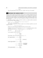
3.4.3 Central Differences
The central difference operator is denoted by the symbol δ and central differences is given by,
() ( ) ( ) or
22
hh
fx fx fxδ=+−−
x
y
δ
=
+−
−
,
22
hh
xx
yy
or
1/2
yδ
= y
1
– y
0
3/2

yδ
=

y
2
– y
1

−
δ
1
2
n
y
=
1nn
yy
−
−
Central Difference Table:
δδ δ δ
δ
δ
δδ
δδ
δδ
δ
δ
234
00

1/2
2
11 1
3
3/2 3/2
24
22 2 2
3
5/2 5/2
2
33 3
7/2
44
xy
xy
y
xy y
yy
xy y y
yy
xy y
y
xy
3.4.4 Other Difference Operators
(a) The Operator E: The operator E is called shift operator or displacement or translation
operator. It shows the operation of increasing the argument value x by its interval of differencing
h so that.
CALCULUS OF FINITE DIFFERENCES
113
Ef (x) = f(x + h) or Ey

x
= y
x+h
Similarly, Ef(x + h)= f(x + 2h)

In general,
n
x
Ey
=
or ( ) ( )
n
xnh
y Efx fx nh
+
=+
In the same manner, E
–1
f(x)= f(x – h)
Also, E
–2
f(x)= f(x – 2h)
E
–n
f(x)= f(x – nh)
This is called inverse of shift operator.
(b) Differential Operator D: The differential operator for a function y = f(x) is defined by
()Df x
=
()

d
fx
dx
2
()
Dfx
=
2
2
()
d
fx
dx
and so on.
The operator ∆ is an analogous to the operator D of differential calculus. In finite differences,
we deal with ratio of simultaneous increments of mutually dependent quantities where as in
differential calculus, we find the limit of such ratios when the increment tends to 0.
(c) The Unit Operator 1: The unit operator 1 has a property that 1. f(x) = f(x). It is also called
identity operator.
(d) Averaging Operator
µµ
µµ
µ: The operator µ is a averaging operator and is defined by,
µy
x
=
+−

+




22
1
2
hh
xx
yy
i.e.,
()fxµ
=

++ −


1
()()
22 2
hh
fx fx
3.4.5 Properties of Operators
1. The operators
,,,, and ED∆∇ δµ
are all linear operators.
i.e.,
∇
(af (x + h) + bφ(x + h)= [af (x + h)+bφ(x + b)] – [af (x) + bφ(x)]
= a[f(x + h) – f(x)] + b[φ(x + h) – φ(x)]
= a
∇

f(x + h) + b
∇
φ(x+h)
Hence,
∇
is a linear operator.
On substituting a = 1, b = 1, we get

∇
[f(x + h) + φ(x + h)] =
∇
f(x + h) +
∇
φ(x + h)
Also on substituting b = 0, we get
∇
[af(x + h)], = a
∇
f(x + h)
2. The operator is distributive over addition.
3. All the operators follows the law of indices. i.e.,
114
COMPUTER BASED NUMERICAL AND STATISTICAL TECHNIQUES
∆
p
∆
q
f(x)= ∆
p+q
f(x) = ∆

q
∆
p
f(x)
Also, ∆[ f(x) + φ(x)] = ∆[φ(x) + f(x)]
4. E and ∆ are not commutative with respect to variables.
5. If f(x) = 0, then it does not mean that either ∆ = 0 or f(x) = 0.
6. Operators E and ∆ cannot stand without operands.
3.4.6 Relation between Different Operators
There are few relations defined between these operators. Some of them are:
1.
∇
= 1 – E
–1
or E = (1 –
∇
)
–1
2.
∆
= E – 1 or E = 1 +
∆
3. E
∇
=
∇
E =
∆
4. E = e
hD

= 1 +
∆
, where D is the differential operator.
5.
δ
= E
1/2
– E
–1/2
6.
µ
=
1
2
(E
1/2
+ E
–1/2
)
7.
δ
E
1/2
=
∆
Proof:
3. (E
∇
) f(x)= E{
∇

f(x)} = E{f(x) – f (x – h)}
= Ef (x) – Ef (x – h)
= f (x + h) – f(x) =
∆
f (x) (1)
Also, (
∇
E) f(x)=
∇
{Ef (x)} =
∇
f (x + h)
= f(x + h) – f(x) = ∆f(x) (2)
From (1) and (2), we get E
∇
=
∆
and
∇
E =
∆
⇒
E
∇
=
∇
E =
∆
.
4. Ef (x)= f (x + h)

= f(x) + h
′
f
(x) +
2
2!
h

′′
f
(x) + (By using Taylor’s theorem)
= 1.f(x) + hDf (x) +
2
2!
h
D
2
f (x) +
= e
hD
f (x)
Ef (x)= e
hD
f(x) or E = e
hD
Since, E = 1 +
∆
, therefore
∆
= e

hD
– 1.
5.
δ
y
x
= y
+
2
h
x

– y
x –
2
h

= E
1/2
y
x
– E
–1/2
y
x
= (E
1/2
– E
–1/2
)y

x
Therefore,
δ
= E
1/2
– E
–1/2
6.
µ
y
x
=
1
2

22
hh
xx
yy
+−

+


=
1
2
(E
1/2
y

x
+ E
–1/2
y
x
)
=
1
2
(E
1/2
+ E
–1/2
)y
x
CALCULUS OF FINITE DIFFERENCES
115
Therefore,
µ
=
1
2
(E
1/2
+ E
–1/2
)
7.
δ
E

1/2
y
x
=
δ
y
x+h


=
2
h
x
y
+
– y
x
=
∆
y
x
Therefore,
δ
E
1/2
=
∆
.
Example 12. Show that:
(a) (E

1/2
+ E
–1/2
) (1 + ∆)
1/2
= 2 + ∆
(b) ∆ =
1
2
δ
2
+
δ
+δ
2
14
Sol. (a) Since 1 +
∆
= E therefore
(E
1/2
+ E
–1/2
) E
1/2
= E + 1 = 1 +
∆
+ 1 =
∆
+ 2.

(b)
22
1
1/4
2
δ+δ +δ
=
1
2
(E
1/2
– E
–1/2
)
2
+ (E
1/2
– E
–1/2
)
()
2
1/2 1/2
1
1
4
EE
−
+−
=

1
2
(E + E
–1
–2) + (E
1/2
– E
–1/2
)
1/2 1/2
2
EE
−

−



=
1
2
(2E – 2) = E – 1 = ∆
Example 13. Prove that (1) ∆ +
∆∇
∇= −
∇∆
(2) (1 + ∆) (1 –
∇
)
≡

1
Where
∆
and
∇
are forward and backward difference operators respectively.
Sol. (1)
∆∇

−

∇∆

y
x
=
1
1
11
1
1
EE
E
E
−
−

−−
−



−
−

y
x
=
1
1
1
1
E
E
E
E
E
E

−



−


−
−
−






y
x
=
1
E
E

−


y
x
= (E – E
–1
)y
x
= {(1 +
∆
) – (1 –
∇
)} y
x
= (
∆
+
∇
) y

x
Hence,
∆∇
−
∇∆
=
∆
+
∇
.
(2) (1 +
∆
) (1 –
∇
) y
x
= (1 +
∆
) [y
x
–
∇
y
x
]
= (1 +
∆
) [y
x
–{y

x
– y
x–h
}] = (1 +
∆
) [y
x –h
]
= E(y
x – h
) = EE
–1
y
x
= 1. y
x
(the interval of differencing being 1)
Hence, (1 + ∆) (1 –
∇
) ≡ 1.