A textbook of Computer Based Numerical and Statiscal Techniques part 31 docx

286
COMPUTER BASED NUMERICAL AND STATISTICAL TECHNIQUES
1. S(x
i
) = f(x
i
); i = 0, 1, 2, n
2. On each subinterval [x
i–1
,x
i
], 1
≤
i
≤
n, S(x) is a polynomial in n of degree at most n .
3. S(x) and its (n –1) derivatives are continuous on [a, b].
4. S(x) is a polynomial of degree one for x < a and x > b.
The process of constructing such type of polynomial is called spline interpolation.
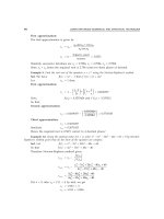
5.7.4 Cubic Spline Interpolation for Equally and Unequally Spaced Values
According to the idea of draftsman spline, it is required that both
dy
dx
and the curvature
2
2
dy
dx
are
the same for the pair of cubic that join at each point. The cubic spline have possess the following
properties:

1. S(x
i
) = f
i
, i = 0, 1, 2, ,n.
2. The cubic and their first and second derivatives are continuous i.e., S(x), S
I
(x) and S
II
(x)
and continuous on [a, b]
3. On each subintervals [x
i–1
, x
i
] 1
≤
i
≤
n, S(x) is a third degree polynomial.
4. The third derivatives of the cubics usually have jumps discontinuities at the ducks or the
junction points.
Y
P
0
f(x )
1
P
1
Ducks

f(x )
2
P
2
x
0
x
1
x
2
x
i
x
i + 1
x
i + 2
x
n – 1
x
n
X
f(x )
i
f(x )
i + 1
P
i
P
i + 1
Spline curve

f(x )
i + 2
P
i + 2
P
n – 1
f(x )
n – 1
f(x )
n
P
n
FIG. 5.4
Where x
i
= for i = 0, 1, 2 , n may or may not be equally spaced.
Let a cubic polynomial for the i
th
interval is
S(x
i
)= a
i
(x – x
i
)
3
+ b
i
(x – x

i
)
2
+ c
i
(x – x
i
) + d
i
(1)
Since this polynomial is valid for both the points x
i
and x
i+1
therefore,
S(x
i
)= a
i
(x
i
– x
i
)
3
+ b
i
(x
i
– x

i
)
2
+ c
i
(x
i
– x
i
) + d
i
(2)
⇒ S(x
i
)= d
i
S(x
i+1
)= a
i
(x
i+1
– x
i
)
3
+ b
i
(x
i+1

– x
i
)
2
+ c
i
(x
i+1
– x
i
) + d
i
⇒
()
1i
Sx
+
=
32
1
1l
i
ii i ii i
ah bh ch d
+
++
+++
(3)
where h
i + 1

= x
i + 1
– x
i
.
INTERPOLATION WITH UNEQUAL INTERVAL
287
Now, Twice differentiate Equation (1) we get,
S’ (x
i
)= 3a
i
(x – x
i
)
2
+ 2b
i
(x – x
i
) + c
i
(4)
S’’(x
i
)= 6a
i
(x – x
i
)

4
+ 2b
i
(5)
Now, Let P
i
= S’’ (x
i
) then equation (5) becomes
P
i
= 6a
i
(x – x
i
) + 2b
i
at x = x
i
,
P
i
= 2b
i

2
i
i
P
b

⇒=
(6)
at x = x
i+1
,
P
i + 1
= 6a
i
(x
i + 1
– x
i
) + 2b
i
P
i + 1
= 6a
i
(x
i+1
– x
i
) + P
i
[using (6)]
P
i + 1
= 6a
i

h
i+1
+ P
i
a
i
=
1
1
6
ii
i
PP
h
+
+
−
(7)
Now substituting the values of d
i
, a
i
and b
i
from (2), (6) and (7) in (3)
()
1i
Sx
+
=

()
()
1
32
1
11
1
1
62
i
i
i
ii ii i
i
P
PPh h ch sx
h
+
+
++
+
−+ ++
()
1i
Sx
+
=
()
()
2

1
2
1
11
62
i
i
i
ii ii i
P
h
PP h ch sx
+
+
++
−+++
()
1i
Sx
+
=
()
21
1
1
62
ii
i
i
iii

PP
P
Sx h ch
+
+
+
−

++


()
1i
Sx
+
=
()
()
2
l
11
3
6
i
iiiiii
h
Sx P P P ch
+
++
=−++

c
i
=
()
()
[]
2
1
l
1
1
3
6
ii
i
iii
i
Sx Sx
h
PPP
h
+
+
+
+
−
−−+
c
i
=

()
()
[]
1
l
1
1
2
6
ii
i
ii
i
Sx Sx
h
PP
h
+
+
+
+
−
−+
(8)
Now, the slope at the point x
i
(because the curve has equal slope at the point [x
i
, S(x
i

)]
hence from equation (4).
S’ (x
i
)= 3a
i
(x
i
– x
i
)
2
+ 2b
i
(x
i
– x
i
) + c
i
()
ii
Sx c
′
⇒=
(9)
c
i
= S’ =
()

()
1
1
1
6
ii
i
i
Sx Sx
h
h
+
+
+
−
−

1
2
ii
PP
+

+

(10)
But S’ (x
i
) for the last subinterval is,
S’ (x

i
)= 3a
i–1
h
2
i
+ 2b
i–1
h
i
+ c
i–1
. (11)
and after using a
i–1
, b
i–1
, and c
i–1
S’ (x
i
)= 3
[]
()
()
[]
11
2
11 1
11

2. 2
62 6
i
i
ii i ii i i
ii
Sx Sx
h
PP h Ph P P
hh
−
−− −
+
−+ + −−
288
COMPUTER BASED NUMERICAL AND STATISTICAL TECHNIQUES
S’ (x
i
)=
()
()
1
1
2
6
ii
ii
i
i
Sx Sx

PP
h
h
−
−
+
+
+
(12)
For equation (9) and (10)
c
i
= 3a
i–1
= h
i
2
+ 2b
i–1
h
i
+ c
i–1
On substituting the values of a
i–1
, b
i–1
, c
i–1
and c

i
()
()
()
() ( )
1
11
1
1
2
2
666
ii
iih
iiii
ii
ii
Sx Sx
Sx Sx
hPhP
PP
hh
+
−
+−
+
+
−
−
−+= ++

()()
()
()
()
1
1
11
1
1
2
2
666
ii
ii
iiiii
ii
ii
Sx Sx
Sx Sx
hPhPh
PP
hh
−
+
+−
+
+
−
−

−=+++

()
()
()
()
()
1
1
11
1
1
1
636
ii
ii iii
ii
ii
ii
Sx Sx
Sx Sx h h P
hP
hP
hh
−
+
++
−
+
−

+− +
−=++
for i = 1, 2, n – 1
⇒
()
()()() ( )
11
11 1 1
1
26
iiii
ii i ii ii
ii
Sx Sx Sx Sx
hP h hP hP
hh
+−
++ + −
+
−−
+++= −


(13)
Now for equally spaced argument i.e., h
i
= h Equation (13) becomes

[]
() ()()

11 1 1
6
42
4
iii i i i
hP P P Sx Sx Sx
+− + −
++ = − +


or P
i+1
+ 4P
i
+ P
i – 1
=
2
6
h
[S(x
i + 1
) – 2S (x
i
) + S(x
i–1
)] (14)
while the S(x) for equally spaced becomes.
()
() ( ) ()

2
33
11 1
11
1)
66
ii ii i i i
h
Sx x x P x x P x x Sx P
hh
−− −



=−+− +− −−






+
()
()
2
1
1
6
iii
h

xx Sx P
h
−

−−


(15)
Equation (15) gives cubic spline interpolation while equation (14) gives the condition for P
i
.
Remarks:
(1) If
0
= P = 0
n
P
; it is called free boundary conditions and the spline curve for this condition
is called the natural spline because the splines are assumed to take their natural straight
line shape outside the interval of approximation.
(2) If
=
0+11
= P , P
nn
PP
;
01111
= , ,
nn n

fff f hh
++
==
then spline is called periodic splines.
(3) For a non-periodic spline we use.
0
'( ) , ( )
n
fa f fb f
′′ ′
==
⇒
0
01 0

6
2 + =
i
i
ff
PP f
hh

−
′
−


⇒
1

1

6
+ 2 =
nn
nn n
nn
ff
PP f
hh
−
−

−
′
−


INTERPOLATION WITH UNEQUAL INTERVAL
289
Example 1. Obtain cubic spline for every subinterval, given in the tubular form.
()
x0123
f x 1 2 33 244
With the end conditions M
0
= 0 = M
3
Sol. Here, we have equal spaced intervals as h
1

= h
2
= h
3
= 1, hence the condition for M
i
becomes.
()
()
()
111
1
462 1,2
iiiiiii
MMM fx fxfx
−+−
+
++= − + =

⇒
() ()
()
012 2 1 0
462
MMM fx fxfx
++= − +


⇒
()

() ()
123 3 2 1
462
MMM fx fxfx
++= − +

Now, after substituting the values of f(x
i
) and M
0
= 0 = M
3
we get

12 1 2
4 180 4 1080
MM andM M+= + =

12
24 276
MandM=− =
x
0
= 0 x
1
= 1 x
2
= 2 x
3
= 3

h
1
= 1 h
2
= 1 h
3
= 1
t
0
= 1 t
1
= 2 t
2
= 33 t
3
= 244
Now, the corresponding cubic spline can be obtained by having
()
() ( ) ()
33
11
11
6
ii iii
fx x x M x x M x x
hh
−−

=− +− +−


()
()
()
2
2
11 1
1
, 1,2,3
66
ii iii
h
h
fx M x x fx M i
h
−− −


−+− − =




Now, for i = 1 (the interval is [0, 1]), f(x) = – 4x
3
+ 5x + 1
Similarly, for [1, 2], f(x) = 50x
3
– 162x
2
+ 167x – 53 and for [2, 3],

f(x) = – 46x
3
+ 414x
2
– 985x + 715.
Example 2: Find the cube splines for following data:
()
x:0123
fx :12511
with the end condition M
0
= 0 = M
3
and also calculate f (2.5)and f’(2.5).
Sol. Here intervals are equally spaced with difference 1 and n = 3. Now, the condition for
M
i
is
() ()()
111 1
462 1,2
iii i ii
MMM fx fxfxi
−++ −
++ = − + =


⇒
()
() ()

012 0 1 2
462
MMM fx fxfx
++= − +


290
COMPUTER BASED NUMERICAL AND STATISTICAL TECHNIQUES
⇒
() ()
()
123 1 2 3
462
MMM fx fxfx
++= − +


but M
0
= 0 M
3
then it becomes

12 1 2
412418
MM andM M+= = =
M
1
= 2 and M
2

= 4
Now, the corresponding cubic spline can be obtained by having

()
() ( ) ()
33
11
1
6
ii iii
fx x x M x x M x x
h
−−

=− +− +−

()
()
()
1
11
, 1,2,3
66
ii
iii
MM
fx x x fx i
−
−−


−+− − =


Now, for i = 1 (the interval is [0, 1])
f(x) =
()
3
1
23
3
xx
++
Similarly, for [1, 2] f(x) =
1
3
(x
3
+ 2x + 3) and for [2, 3], f(x) =
1
3

()
−+ − +
32
2183427
xx x
Now, f(2.5) = 7.66 and f ’ (2.5) = 6.16
Example 3. Obtain the cubic spline for the following data:
()
x:0123

fx : 2 6 8 2
−−
Sol. Take initial conditions M
0
= 0 = M
3
for i = 1, 2 n
h
2
[M
i–1
+ 4M
i
+ M
i+1
] = 6 [f
i+1
– 2f
i
+ f
i–1
]
Here, h = 1;
∴
()
012 210
46201
MMM fffforx
++=−+ ≤≤

()
123321
46212
MMM f ffforx
++=−+ ≤≤

++=


++=

210
321
436
472
MMM
MMM
Using initial conditions, we get
M
1
= 4.8,M
2
= 16.8
Hence for 0
≤
x
≤
1 spline is given by
S (x)=
() () ()( )()( )

33
0100 11
1
101606
6
xM x M x f M x f M

−+−+−−+−−

=
()
()
()
()
3
1
4.8 1 12 36 4.8
6
xxx

+− +−−

=
3
0.8 8.8 2
xx−+
Hence for 1
≤
x
≤

2 spline is given by
S(x)= 2x
3
– 3. 6x
2
– 5.2x + 0.8
Similarly, for 2
≤
x
≤
3
S(x) = –2.8x
3
+ 25.2x
2
– 62.8x + 39.2. Ans.
INTERPOLATION WITH UNEQUAL INTERVAL
291
Example 4. Estimate the function value f at x = 7 using cubic splines from the following data: Given
P
2
= P
0
= 0.
i
i
i012
x4916
f234
Sol. h

1
= x
1
– x
0
= 9 – 4 = 5
h
2
= x
2
– x
1
= 16 – 9 = 7
()()
12
12
0122110
21
11
633
hh
hh
PPPffff
hh
+
++=−−−
⇒
1
1
70

P =−
= – 0.0143
Since, n = 3 therefore, there are two cubic splines given by
S
1
(x) = x
0
≤
x
≤
x
1
S
2
(x) = x
1
≤
x
≤
x
2

()
() ( )
{}
33
11
1
6
ii ii

i
Sx x x P x x P
h
−−
=−+−
() ()
2
2
11 1
11
66
i
i
ii i iii
ii
h
h
xxf P xx f P
hh
−− −





+− − +− −












For i = 1
S(x) =
()
()
{}
()
2
33
1
10 01 100
11
11
66
h
xxP xx P xxf P
hh



−+− + −−







()
2
1
01 1
1
1
6
h
xx f P
h



+−−







()
() ()
143
27 0.0143 3 25 0.0024
30 5 5
Sx

=− +++×


()
7 2.64862S
=
. Ans.
PROBLEM SET 5.5
1. Using the Chebyshev polynomials T
n
(x), obtain the least square approximation of degree
eleven for f(x) = cos
–1
x.
() () () () ()
01 3 5
44 4

2925
fx Tx Tx Tx Tx
π

=−− −

ππ π

Ans.
() () ()
711
44 4

9
49 81 121
Tx T x T x

−−−

ππ π

2. Find the linear least-squares polynomial approximation to the function f(x) = 5 + x
2
on the
interval [0, 1].
()
1
29 6
6
yx

=+


Ans.
3. Find the quadratic least squares polynomial approximation to the function f(x) = x
3/2
on the
interval [0, 1].
()
2
1
248 60

105
yxx

=−++


Ans.
292
COMPUTER BASED NUMERICAL AND STATISTICAL TECHNIQUES
4. Using the Chebyshev polynomials T
n
(x), obtain the least squares approximation of second
degree for f(x) = 4x
3
+ 2x
2
+ 5x – 2 on the interval [1, 1].
[Ans. f(x) = – T
0
(x) + 8T
1
(x) + T
2
(x)]
5. Find the best lower-order approximation to the cubic 9x
3
+ 7x
2
, –1 ≤ x ≤ 1.
2

27 9
7 , max.error = in [-1,1]
44
xx

+


Ans.
6. Economize the series e
x
2
= 1 + x
2
+
4681012
2 6 24 120 720
xxxx x
+++ +
+ on the interval [–1, 1]
allowing for a tolerance of 0.05. [Ans. e
x
2
= 1.0075 + 0.869x
2
+ 0.8229x
4
]
7. Economize the series x +
35 7

6 120 5040
xx x
++
on the interval [–1, 1], allowing for a tolerance
of 0.0005.
3
383 17
sin
384 96
hx x x

=+


Ans.
8. Find a uniform polynomial approximation of degree 1 to (2x – 1)
3
on the interval [0, 1] so
that the maximum norm of the error function is minimized, using Lanczos economization.
Also calculate the norm of the error function.
Hint: Put x =
1
2
t +
, linear approximation =
()
3
21,
4
x

−
maximum error =
1
4
9. Find the lowest order polynomial which approximates the function f(x) =1 – x + x
2
– x
3
+ x
4
, 0 ≤ x ≤ 1 with an error less than 0.1.
()
2
160 160 131

128 128 128
fx x x

=−+


Ans.
10. Obtain an approximation in the sense of the principle of least squares in the form of a
polynomial of second degree to the function f(x) =
2
1
1
x+
in the range –1
≤

x
≤
1.
[Ans. P (x) =
3
4
(2
π
– 5) +
15
4
(3 – p) x
2
]
11. Find the polynomial of second degree, which is the best approximation in maximum norm
to
x
on the point set
{}
41
0, , , 1,0
99
·
()
2
19
2
16 8
Px x x


=+−


Ans.
12. Find a polynomial P(x) of degree as low as possible such that
()
2
1
max 0.05
x
x
ePx
≤
−≤
[Ans. 1.0075 + 0.8698x
2
+ 0.82292x
4
]
13. Prove that x
2
=
() ()
02
1
2
Tx Tx
+



·
14. Express T
0
(x) + 2T
1
(x) + T
2
(x) as polynomials in x.[Ans. 2x + 2x
2
]
15. Economize the series f(x) = 1 –
23
2816
xx x
−−
·
16. Economize the series cos x = 1 –
24 6
224720
xx x
+−
·
17. Prove that T
n
(x) is a polynomial in x of degree n
18. Find the best lower order approximation to the cubic 5x
3
+ 4x
2
in the closed interval

[–1, 1]. [Ans. 4x
2
+
5
4
x]
INTERPOLATION WITH UNEQUAL INTERVAL
293
19. Find cubic spline for the following data:
()
012 3
12511
x
fx
with end conditions P
0
= 0 = P
3
and also calculate f(2.5), f’(2.5).
20. Estimate the function value f at x = 7 using cubic splines from the following data:
01 2
4916
23 4
i
i
i
x
f
[Ans. S
1

(7) = 2.6229]
21. Fit the following points by the cubic spline:
()
:1234
:15118
x
fx
By using the conditions M
0
= 0 = M
3
. Hence find f(1.5) and f ’(2)
()
32
1
17 51 94 45 1 2
15
fx x x x x


=−+−≤≤



Ans.
()
32
1
55 381 770 53 2 3
15

fx xxx x

=− − − + ≤≤

()
32
1
38 456 1741 1980 3 4
15
fx x x x x

=−+−≤≤


() ()
103 94
1.5 , 2
40 15
ff

′
==


22. Find the cubic spline corresponding to the interval [2, 3] which means the following
representation:
()
:12345
:3015321825
x

fx
with the end condition M
1
= 0 = M
5
and also compute f(2.5), f’(3)
() () ()
32
1
142.9 1058.4 2475.2 1950 2.5 24.03 & 3 2.817
16
fx x x x f f
 

′
=− + − + =− =
 

 
Ans.
23. Fit the following points by Cubic spline and obtain y(1.5):
:1 2 3
:8118
x
y −−
[Ans.
()
3
31412
xx

−+−
()
1.5 5.625y
=−
]
24. Obtain cubic spline approximation valid in the interval [3, 4],
Given that
1234
3102965
x
y
Under the natural spline conditions M(1) = 8 = M(4).
()
{}
32
1
56 72 2092 2175
15
Sx x x x

=− + − +


Ans.
23
62 112
,
55
mm


==


GGG
CHAPTER 6
Numerical Differentiation
and Integration
6.1 INTRODUCTION
The differentiation and integration are losely linked processes which are actually inversely related.
For example, if the given function y(t) represents an objects position as a function of time, its
differentiation provides its velocity,
=() ()
d
vt yt
dt
On the other hand, if we are provided with velocity v(t) as a function of time, its integration
denotes its position.
0
() ()
t
yt vtdt
=
∫
There are so many methods available to find the derivative and definite integration of a
function. But when we have a complicated function or a function given in tabular form, they we
use numerical methods. In the present chapter, we shall be concerned with the problem of numerical
differentiation and integration.
6.2 NUMERICAL DIFFERENTIATION
The method of obtaining the derivatives of a function using a numerical technique is known as
numerical differentiation. There are essentially two situations where numerical differentiation is

required.
They are:
1. The function values are known but the function is unknown, such functions are called
tabulated function.
2. The function to be differentiated is complicated and, therefore, it is difficult to differentiate.
The choice of the formula is the same as discussed for interpolation if the derivative at a
point near the beginning of a set of values given by a table is required then we use Newton
forward formula, and if the same is required at a point near the end of the set of given tabular
294
NUMERICAL DIFFERENTIATION AND INTEGRATION
295
values, then we use Newton’s backward interpolation formula. The central difference formula
(Bessel’s and Stirling’s) used to calculate value for points near the middle of the set of given
tabular values. If the values of x are not equally spaced, we use Newton’s divided difference
interpolation formula or Lagrange’s interpolation formula to get the required value of the
derivative.
6.2.1 Derivation Using Newton’s Forward Interpolation Formula
Newton’s forward interpolation is given by

23
00 0 0
(1) (1)(2)

2! 3!
uu uu u
yy uy y y
−−−
=+∆+ ∆ + ∆
(1)
where

−
=
0
xx
u
h
Differentiating equation (1) with respect to u, we get
−−+
=∆ + ∆ + ∆
2
23
00 0
21 3 62

2! 3!
dy
uuu
yy y
du
(2)
Now
dy
dx
=
dy
du
·
du
dx
=

1
h
dy
du
⋅
Therefore,

−−+−+−
=∆+ ∆+ ∆+ ∆


232
23 4
00 0 0
121362418226

2! 3! 4!
dy
uuuuuu
yy y y
dx h
(3)
As
==
0,
0
xxu
, therefore, putting u = 0 in (3), we get

=



=∆−∆+∆−∆




0
234
0000
1111

234
xx
dy
yyyy
dx h
Differentiating equation (3) again w.r.t. ‘x’, we get

 
==×
 
 
2
2
1
dy dy dy
ddud
du dx dx h du dx
dx

()

−+
=∆+−∆+ ∆−


2
23 4
00 0
2
161811
1
12
uu
yu y y
h
(4)
Putting u = 0 in (4), we get

=


=∆−∆+∆−





0

2
23 2
00 0
22
111

12
xx
dy
yy y
dx h
…(5)
Similarly,

=


=∆−∆+





0
3
34
00
33
13

2
xx
dy
yy
dx h
and so on.