A textbook of Computer Based Numerical and Statiscal Techniques part 50 pptx

476
COMPUTER BASED NUMERICAL AND STATISTICAL TECHNIQUES
Sol. Mean Chart
Mean of 10 sample mean
442
44.2
10 10
x
X ===
∑
Mean Range of 10 sample ranges
58
5.8
10 10
R
R ===
∑
As we have, for
5,n =

2
0.58
A =
,
3
0,
D =

4
2.115
D =

3-σ control limits for x
–
chart are:
2
2
UCL
44.2 0.58 5.8 47.567
LCL
44.2 0.58 5.8 40.836
CL 44.2
x
x
x
XAR
XAR
X
=+
=+×=
=−
=−×=
==
Range Chart: 3-σ Control Limits for R chart are:
4
3
UCL 2.115 5.8 12.267
LCL 0 5.8 0
CL 5.8
R
R
R

DR
DR
R
== ×=
==×=
==
60
50
40
30
20
10
0
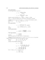
Sample Mean
Mean Chart
0 2 4 6 10 128
Sample Number
FIG. 11.17
From mean chart we see that 2nd, 3rd, 6th and 7th samples lies outside the control limits.
Hence the process is out of control. This shows that some assignable causes of variation
are operating which should be detected and removed.
STATISTICAL QUALITY CONTROL
477
9
8
7
6
5
4
3

2
1
0
Sample Range
0 2 4 6 8 10 12
Sample Number
FIG. 11.18
Since all the points with in the control limits. Hence the process is in statistical control.
Example 2. The following are the mean lengths and ranges of lengths of a finished product from
10 samples each of size 5. The specification limits for length are
±200 5 cm
. Construct x
–
and R-chart
and examine whether the process is under control and state your recommendation.
Sample No. 12345678910
x
201 198 202 200 203 204 199 196 199 201
R 5073472856
Assume for n = 5, A
2
= 0.577, D
3
= 0, D
4
= 2.115.
Sol. In given problem specification limits for length are given 200 ± 5 cm. Hence standard
deviation is unknown.
(1) Control Limits for x
–

-chart are:
Central limit,
CL
x
= µ = 200

2
UCL 200 0.577 4.7
x
AR
=µ+ = + ×

202.712=
;
47
10 10
R
R ==
∑

2
LCL 200 0.577 4.7
x
AR
=µ− = − ×
= 197.288
4.7R =
(2) Control limits for R-Chart are:

4

3
UCL 9.941 2.115 4.7
CL 4.7
LCL 0 0 4.7
R
R
R
DR
R
DR
===×
==
== =×
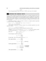
from control charts for mean and range, the process is in statistical control in R
—
-Chart because
all points lies with in the control limits where as in x
—
-chart, process is out of control because
sample 5, 6 and 8 lies outside the control limits. The process therefore should be halted to check
478
COMPUTER BASED NUMERICAL AND STATISTICAL TECHNIQUES
whether there are any assignable causes. If assignable causes found, the process should be
re-adjusted to remove assignable cause.
205
204
203
202
201
200

199
198
197
196
195
Sample Mean
0 2 4 6 8 10 12
Sample Number
Mean Chart
FIG. 11.19
Range Chart
10
8
6
4
2
0
Sample Range
0 5 10 15
Sample Number
FIG. 11.20
Example 3. In a glass factory, the task of quality control was done with the help of mean (x
—
) and
standard deviation σ charts. 18 samples of 10 items each were chosen and then values ∑X and ∑S were
found to be 595.8 and 8.28 respectively. Determine the 3-σ limits for mean and standard deviation chart.
Given that n = 10, A
1
= 1.03, B
3

= 0.28, B
4
= 1.72, ∑S = 8.28.
Sol.
No. of samples 18
S
—
=
∑
18
S
=
8.28
18
= 0.46
hence, 3-σ control limits for standard deviation chart are:
UCL
–
S
= B
4
.S
—
= 1.72 × 0.48 = 0.7912
LCL
S
–
= B
3
.S

—
= 0.28 – 0.46 = 0.1288
CL
S
–
= 0.46
3-σ control limits for mean chart (x
—
) are:
X
—
=
∑
18
x
=
595.8
18
= 33.1
STATISTICAL QUALITY CONTROL
479
UCL
X
—
= x
—
+ A
1
σ
= 33.1 + 1.03 × 0.46

UCL
X
—
= 33.57
LCL
X
—
= x
—
– A
1
σ
= 33.1 – 1.03 × 0.46
LCL
X
—
= 32.63
CL
X
—
= 33.1.
Example 4. If the average fraction defective of a large sample of a product is 0.1537, calculate
the control limits when subgroup size is 2,000.
Sol. Here, Sample size n = 2,000 for each sample
Average fraction defective = 0.1537 i.e., P = 0.1537
⇒ Q =1 – P = 1 – 0.1537
Q = 0.8463
Hence, 3–σ control limits for P-Chart are :
± 3
PQ

P
n
UCL
P
=
×
+
0.1537 0.8463
0.1537 3
2, 000
UCL
P
= 0.1537 + 0.02418 = 0.17788
LCL
P
=
×
−
0.1537 0.8463
0.1537 3
2, 000

LCL 0.1537 0.02418 0.12952
P
=− =

CL 0.5137
P
= .
Example 5. The following data gives the number of defectives in 10 independent samples of

varying sizes from a production process.
Sample no. 12345678910
Sample size 2000 1500 1400 1350 1250 1760 1875 1955 3125 1575
No. of defectives 425 430 216 341 225 322 280 306 337 305
Draw the control chart for fraction defective.
Sol. (In problem 4 sample size is fixed whereas in this problem sample size is variable)
Since it is a problem of variable sample size so control chart for fraction defective can be
drawn in two ways.
(1) By first way, we set up two sets of control limits, one based on the maximum sample
size,
3125n =
and the second based on minimum sample size
1, 250.n =
(a) For
3, 125;n =

UCL 0.200,=

LCL 0.159=
(b) For
1, 250;n =

UCL 0.212,=

LCL 0.147=
480
COMPUTER BASED NUMERICAL AND STATISTICAL TECHNIQUES
12
10
8

6
4
2
0
Number of Defectives
0 100 200 300 400 500
Sample Number
FIG. 11.21 Control Chart for Fraction Defective
Since there are 4 points lies outside (based on minimum sample size) of control limits,
so process is of out of control.
(2) By second way, 3-
σ
limit for each sample separately obtained by using formula
3
PQ
P
n
±
where
Total no. of defectives
Total sample size
d
P
n
==
∑
∑
and
n
is corresponding sample size.

3187
0.1791 1 0.8209
17790
d
PQP
n
∑
== = ⇒=−=
∑
∴
()
PQ
= 0.1791 × 0.8209 = 0.1470231
nn
nn
n
dd
dd
d
P = d/nP = d/n
P = d/nP = d/n
P = d/n
1/n1/n
1/n1/n
1/n
P Q
n
P Q
n

3 × 3 ×
3 × 3 ×
3 ×
P Q
n
UCLUCL
UCLUCL
UCL
LCLLCL
LCLLCL
LCL
2000 425 0.2125 0.0005 0.000735 0.008573 0.025719 0.205 0.153
1500 430 0.2867 0.00066 0.000098 0.009899 0.029698 0.209 0.149
1400 216 0.1543 0.00071 0.000105 0.010247 0.030741 0.210 0.148
1350 341 0.2526 0.00074 0.000109 0.010440 0.031321 0.210 0.148
1250 225 0.1800 0.00080 0.000118 0.010863 0.032588 0.212 0.147
1760 322 0.1829 0.00057 0.000084 0.009138 0.027413 0.207 0.152
1875 280 0.1495 0.00053 0.000078 0.008854 0.026562 0.206 0.153
1995 306 0.1565 0.00051 0.000075 0.008672 0.026015 0.205 0.153
3125 337 0.1078 0.00032 0.000047 0.006856 0.020567 0.200 0.159
1575 305 0.1937 0.00063 0.000093 0.009659 0.028977 0.0208 0.150
17790 3187
STATISTICAL QUALITY CONTROL
481
500
400
300
200
100
0

Number of Defectives
0 1000 2000 3000 4000
Sample Size
Sample points corresponding to sample no. 1, 2, 4, 7 and 9 lie
outside the control limits. Hence, process is out of control.
FIG. 11.22
Example 6. A daily sample of 30 items was taken over a period of 14 days in order to establish
attributes control limits. If 21 defectives were found, what should be upper and lower control limits of
the proportion of defectives?
Sol. Since a sample of 30 items is taken daily over a period of 14 days.
Total No. of items inspected = 30 × 14 = 420
No. of defective found = 21
n = 30
∴Average fraction defective P
—
=
21
420
= 0.05
∴ UCL
P
=
3
PQ
P
n
+
where
1QP=−
=

()
()
1
0.05 0.95
30.053
30
PP
P
n
−
×
+=+
UCL
P
= 0.05 + 3 × 0.0398
UCL
P
= 0.1694
LCL
P
=
()
1
3
PP
P
n
−
−
= 0.05 – 0.1194 < 0 (negative)

∴ LCL
P
= 0.
Example 7. The past record of a factory using quality control melthods show that on the average
4 articles produced are defective out of a batch of 100. What is the maximum number of defective articles
likely to be encountered in the batch of 100, when the production process is in a state of control?
Sol. n = Sample size = 400
P = Process fraction defective =
4
100
= 0.04
Q = 1 – P = 0.96
482
COMPUTER BASED NUMERICAL AND STATISTICAL TECHNIQUES
Let d be the number of defectives in a sample size of n. i.e., np. The 3–σ limit for number
of defectives are given by
() ()
3.Ed sEd
±
or
3np nPQ±
400 0.04 3 400 0.04 0.96=× ± ××
16 3 15.36 16 3 3.9192=± =±×
16 11.7576=±
()
4.2424, 27.7576
=
Therefore if the production process is in a statistical control, the number of defective items
to be encountered in a batch of 400 should lie within the control limits, viz. (4.2424, 27.7576),
i.e., (4, 28). Hence the maximum number of defective items in this batch is 28.

Example 8. In a blade manufacturing factory, 1000 blades are examined daily. Following information
shows number of defective blades obtained there. Draw the np-chart and give your comment?
1 2 3 4 5 6 7 8 9 10 11 12 13 14 15
.
910128715101210 8 7 13141516
Date
No of
Defective
Sol. Here
10000,n =
15k =
(sample no.)
If
P
denotes the fraction defectives produced by the entire process then

166
0.011
15 1000
P
P
kn
∑
== =
×
∴

1000 0.011 11np =× =
Hence control limits are
()

()
()
CL 11
UCL 3 (1 )
11 3 11 1 0.011
UCL 20.894
LCL 3 1
11 3 11 1 0.011
LCL 1.106
np
np np p
np np p
==
== −−
=+ −−
=
=− −−
=− −−
=
Since all the 15 points lies within the control limits, the process is under control.
STATISTICAL QUALITY CONTROL
483
20
15
10
5
0
No. of defectives
0 5 10 15 20
Date

FIG. 11.23
Example 9.


The number of mistakes made by an accounts clerk is given below:
Week 1234567891011121314151617181920
No.ofMistakes10201010123310071010
Establish a suitable control chart and state how it should be used in future in order to control the
mistakes of the clerk.
Sol. The control chart to be used for the given problem is the number of defects chart i.e.,
C-chart.
Average no. of mistakes.
c
—
=
24
1.2
20 20
C∑
==
Thus the control limits for c
—
-chart are;
(i) UCL =
3cc+
=
1.2 3 1.2+
= 4.49
(ii) CL = c
—

= 1.2
(iii) LCL =
3cc−
=
1.2 3 1.2−
= 2.09 ≈ 0
3 The number of mistakes during the 16th week lies outside the UCL the process is not
under control.
Now to establish the suitable control chart for future, we homogenize the data for future
control by eliminating the data corresponding to the 16th week.

17
0.895.
19
new
C
==
Hence the revised control limits for
c
chart are:
UCL 3 0.895 3 0.895 3.73
LCL 3 0.895 3 0.895 1.94 0
17
CL 0.895.
19
cc
cc
C
=+ = + =
=− = − =− ≅

== =
484
COMPUTER BASED NUMERICAL AND STATISTICAL TECHNIQUES
So the revised C-chart for revised control limit is in statistical control, i.e., all the points
lies within the control limits.
8
6
4
2
0
No. of Mistakes
Week
FIG. 11.24
Example 10. During the examination of equal length of cloth, the following are the number of
defects observed.
2340567432
Draw a control chart for the number of defects and comment whether the process is under control
or not?
Sol. Let the no. of defects per unit (equal length) be denoted by c.
The average no. of defects in 10 samples

36
3.6
20 10
c
c
∑
===
Hence 3–σ limit for c-chart are:

3cc±

3.6 3 3.6=±

3.6 3 1.8974=±×

3.6 5.6922=±
UCL
C
–

= 3.6 + 5.6922 = 9.2922
LCL
C
–
= 3.6 – 5.6922 = – 2.0922 ≈ 0
CL
C
–
= 3.6
(LCL
C
–
= 0 because no. of defects per unit cannot be negative)
STATISTICAL QUALITY CONTROL
485
8
6
4
2

0
Number of Defect
0 2 4 6 8 10 12
Sample Number
FIG. 11.25
Since all the points are within the control limits therefore the process is in statistical
control.
Example 11. An automobile producer wishes to control the number of defects per automobile. The
data for 16 such automobiles is shown below:
Sample No. 12345678910111213141516
No. of defects243218105 2 313412
1. Set up the control lmits for c-charts.
2. Do these data come from a controlled process ? If not, calculated the revised control charts
limits.
Sol. Here k = 16
Average no. of defects in 16 units

142
2.625
16
cC
k
=∑= =
Thus, the control limits for c-chart are:
UCL =
3 2.625 3 2.625 2.625 4.861 7.486cc+=+ =+=
CL =
2.625c =
LCL =
3 2.625 3 2.625 2.625 4.861 2.236 0cc−= − = − =− ≈

10
8
6
4
2
0
No. of Defect
Sample Number
FIG. 11.26