A textbook of Computer Based Numerical and Statiscal Techniques part 54 potx
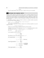
Bạn đang xem bản rút gọn của tài liệu. Xem và tải ngay bản đầy đủ của tài liệu tại đây (123.87 KB, 10 trang )
516
COMPUTER BASED NUMERICAL AND STATISTICAL TECHNIQUES
where
x
1
be the mean of a sample of size n
1
from a population with mean µ
1
and variance σ
1
2.
x
2
be the mean of an independent sample of size n
2
from population with mean µ
2
and
variance σ
2
2
.
Remarks:
1. Under the null hypothesis H
0
: µ
1
= µ
2
, i.e., there is no significant difference
between the sample means therefore σ
1
2
= σ
2
2
= σ
2
i.e., if the sample have been drawn from the
populations with common standard deviation σ then
Z =
xx
nn
1
2
12
11
–
σ+
2. If σ
1
2
≠ σ
2
2
and σ
1
and σ
2
are not known, then test statistic estimated from sample values. i.e.,
Z =
xx
S
n
S
n
1
2
1
2
1
2
2
2
–
F
H
G
I
K
J
+
F
H
G
I
K
J
3. If σ
is not known, then its test statistic based on the sample variances is used.
If σ
1
= σ
2
, we use σ
2
=
nS nS
nn
11
2
22
2
12
+
+
to evaluate σ.
Test statistic Z =
12
22
11 22
12 1 2
11
xx
nS nS
nn n n
−
+
+
+
(E) Test of Significance for the Difference of standard Deviations: If S
1
and S
2
are
the standard deviations of two independent samples, then under the null hypothesis,
H
0
: σ
1
= σ
2
(the sample S.D. do not differ significantly), the test statistic is given by
Z =
SS
SE S S
12
12
–
–
bg
(For large samples)
but the difference of the sample standard deviation is given by
S.E. (S
1
– S
2
)=
σσ
1
2
1
2
2
2
22
nn
+
∴ Z =
SS
nn
12
1
2
1
2
2
2
22
−
+
σσ
when σ
1
2
and σ
2
2
are not known (i.e., population S.D. are not known) then the test statistic reduces
to
Z =
SS
S
n
S
n
12
1
2
1
2
2
2
22
–
+
TESTING OF HYPOTHESIS
517
Example 25. Intelligence tests were given to two groups of boys and girls
Mean S.D. Size
Girls 75 8 60
Boys 73 10 100
Examine if the difference between mean scores is significant.
Sol. Null hypothesis H
0
: There is no significant difference between mean scores i.e.,
x
—
1
= x
2
.
H
1
: x
—
1
= x
—
2
Under the null hypothesis Z =
xx
S
n
S
n
12
1
2
1
2
2
2
–
+
F
H
G
I
K
J
=
75 73
8
60
10
100
22
–
+
= 1.3912
Conclusion: As the calculated value of |Z| < 1.96, the significant value of Z at 5% level of
significance, H
0
is accepted.
Example 26. The means of two single large samples of 1000 and 2000 members are 67.5 inches and
68.0 inches respectively. Can the samples be regarded as drawn from the same population of standard
deviation 2.5 inches? (Test at 5% level of significance).
Solution: Given: n
1
= 1000
n
2
= 2000
x
1
= 67.5 inches
x
2
= 68.0 inches
Null hypothesis: H
0
: µ
1
= µ
2
and σ = 2.5 inches
i.e., the samples have been drawn from the same population of standard deviation 2.5
inches.
Alternative hypothesis: H
1
: µ
1
≠µ
2
(Two-tailed)
Test statistic: Under H
0
, the test statistic (For large samples)
Z =
xx
nn
12
2
12
11
–
σ+
F
H
G
I
K
J
Z =
67 5 68 0
25
1
1000
1
2000
.– .
. +
F
H
I
K
=
–.
05
25 00387×
Z = –5.1
Conclusion: Since
Z
> 3, the value is highly significant and we reject the null hypothesis
and conclude that samples are certainly not from the same population with standard deviation
2.5.
Example 27. The average income of persons was Rs. 210 with a S.D. of Rs. 10 in sample of 100
people of a city. For another sample of 150 persons, the average income was Rs. 220 with standard
deviation of Rs. 12. The S.D. of incomes of the people of the city was Rs.11. Test whether there is any
significant difference between the average incomes of the localities.
518
COMPUTER BASED NUMERICAL AND STATISTICAL TECHNIQUES
Sol. Given that n
1
=100, n
2
= 150,
x
1
= 210,
x
2
= 220, S
1
= 10, S
2
= 12.
Null Hypothesis: The difference is not significant. i.e., there is no difference between the
incomes of the localities.
H
0
:
x
1
=
x
2
, H
1
:
x
1
≠
x
2
Under H
0
, Z =
xx
s
n
s
n
1
2
1
2
1
2
2
2
–
+
=
210 220
10
100
12
150
22
–
+
= –7.1428 ∴ |Z| = 7.1428
Conclusion: As the calculated value of |Z| > 1.96, the significant value of Z at 5% level of
significance, H
0
is rejected i.e., there is significant difference between the average incomes of the
localities.
Example 28. In a survey of buying habits, 400 women shoppers are chosen at random in super
market ‘A’ located in a certain section of the city. Their average weekly food expenditure is Rs. 250 with
a standard deviation of Rs. 40. For 400 women shoppers chosen at random in super market ‘B’ in another
section of the city, the average weekly food expenditure is Rs. 220 with a standard deviation of Rs. 55. Test
at 1% level of significance whether the average weekly food expenditure of the two populations of shoppers
are equal.
Sol. We have: n
1
= 400, n
2
= 400,
x
1
= Rs. 250,
x
2
= Rs. 220, S
1
= Rs. 40, S
2
= Rs. 55
Null hypothesis, H
0
: µ
1
= µ
2
i.e., the average weekly food expenditures of the two populations of shoppers are equal.
Alternative Hypothesis, H
1
: µ
1
≠µ
2
(Two-tailed)
Test Statistic: Since samples are large, under H
0
then
Z =
xx
nn
12
1
2
1
2
2
2
–
σσ
+
F
H
G
I
K
J
Since σ
1
and σ
2
are not known then we use
Z =
xx
S
n
S
n
12
1
2
1
2
2
2
–
+
Z =
250 220
40
400
55
400
22
–
af af
+
= 8.82 (Approx.)
Conclusion: Since |Z| is much greater than 2.58, the null hypothesis (µ
1
= µ
2
) is rejected
at 1% level of significance and we conclude that the average weekly expenditures of two
populations of shoppers in market A and B differ significantly.
Example 29. In a certain factory there are two independent processes manufacturing the same items.
The average weight in a sample of 250 items produced from one process is found to be 120 ozs. with a
standard deviation of 12 ozs. While the corresponding figures in a sample of 400 items from the other
process are 124 and 14. Obtain the standard error of difference between the two sample means; Is this
TESTING OF HYPOTHESIS
519
difference significant? Also find the 99% confidence limits for the difference in the average weights of items
produced by the two processes respectively.
Sol. Given: n
1
= 250,
x
1
= 120 ozs, S
1
= 12 ozs = σ
1
n
2
= 400,
x
2
= 124 ozs, S
2
= 14 ozs = σ
2
S.E.
xx
12
–
di
=
σσ
1
2
1
2
2
2
nn
F
H
G
I
K
J
+
F
H
G
I
K
J
=
S
n
S
n
1
2
1
2
2
2
F
H
G
I
K
J
+
F
H
G
I
K
J
=
144
250
196
400
+
F
H
G
I
K
J
=
0 576 0 490 +
= 1.034
Null Hypopthesis, H
0
: µ
1
= µ
2
(i.e., the sample means do not differ significantly)
Altnerative Hypothesis, H
1
= µ
1
≠ µ
2
(Two-tailed)
Test Statistic: Under H
0
, the test statistic is given by
Z =
xx
SE x x
12
12
–
–
di
=
120 124
1 034
–
.
∴ |Z| =
4
1 034.
= 3.87
Conclusion: Since |Z| > 3, the null hypothesis is rejected and we can say that there is
significant difference between the sample means. 99% confidence limits for
µµ
12
–
is
xx
12
–
± 2.58 S.E.
xx
12
–
= 4 ± 2.58 × 1.034
= 4 ± 2.67 (Approx.)
= 6.67 (on taking +ve sign) and 1.33 (on taking –ve sign).
∴ 1.33 <
µµ
12
–
< 6.67
Example 30. Two populations have their means equal, but S.D. of one is twice the other. Show that
in the samples of size 2000 from each drawn under simple sampling conditions, the difference of means will,
in all probability not exceed 0.15σ, where σ is the smaller S.D. what is the probability that the difference
will exceed half this amount ?
Sol. Let standard deviations of the two populations be σ and 2σ respectvely and let µ be
the mean of each of two populations.
Given n
1
= n
2
= 2000
If
x
1
and
x
2
be two sample means then
Z =
xx Exx
SE x x
12 12
12
–– –
–
didi
di
Now E
xx
12
–
di
= E
x
1
di
– E
x
2
di
= µ – µ = 0
(Samples are large)
520
COMPUTER BASED NUMERICAL AND STATISTICAL TECHNIQUES
Also S.E
xx
12
–
di
=
σ
σ
2
1
2
2
2
nn
+
af
=
σ
1
2000
4
2000
+
= 0.05σ
∴ Z =
xx
SE x x
12
12
−
−
di
∼ N (0, 1)
Under simple sampling conditions, we should in all probability have
|Z| <3
⇒
xx
12
–
< 3 S.E.
xx
12
–
di
⇒
xx
12
–
< 0.15 σ
which is the required result.
We want p = P
xx
1
2
1
2
015–.
>×
L
N
M
O
Q
P
σ
∴ p = P [0.05 σ |Z| > 0.075 σ]
3 Z
xx
=
F
H
G
I
K
J
12
005
–
.
σ
= P [|Z| > 1.5]
=1 – P [|Z| ≤ 1.5]
=1 – 2P (0 ≤ Z ≤ 1.5)
= 1 – 2 × 0.4332 = 0.1336. Ans.
Example 31. Random samples drawn from two countries gave the following data relating to the
heights of adult males:
Country A Country B
Males height (in inches) 67.42 67.25
Standard deviation 2.58 2.50
Number in samples 1000 1200
(i) Is the difference between the means significant?
(ii) Is the difference between the standard deviations significant?
Sol. Given: n
1
= 1000, n
2
= 1200,
x
1
= 67.42;
x
2
= 67.25, s
1
= 2.58, s
2
= 2.50
Since the samples size are large we can take
σ
1
= S
1
= 2.58;
σ
2
= S
2
=2.50.
TESTING OF HYPOTHESIS
521
(i) Null Hypothesis: H
0
: µ
1
= µ
2
i.e., sample means do not differ significantly.
Alternative hypothesis: H
1
: µ
1
≠ µ
2
(two-tailed test)
z =
xx
s
n
s
n
12
1
2
1
2
2
2
–
+
=
67 42 67 25
258
1000
250
1200
22
.–.
afaf
+
= 1.56
Since |z| < 1.96 we accept the null hypothesis at 5% level of significance.
(ii) We set up the null hypothesis.
H
0
: σ
1
= σ
2
i.e., the sample S.D.’s do not differ significantly.
Alternative hypothesis: H
1
: σ
1
≠ σ
2
(two-tailed)
∴ The test statistic is
z =
ss
nn
12
1
2
1
2
2
2
22
–
σσ
+
=
ss
s
n
s
n
12
1
2
1
2
2
2
22
–
+
( σ
1
= s
1
, σ
2
= s
2
for large samples)
=
258 250
258
2 1000
250
2 1200
22
..
bg bg
×
+
×
=
008
66564
2000
625
2400
.
.
+
= 1.0387.
Since |z| < 1.96 we accept the null hypothesis at 5% level of significance.
PROBLEM SET 12.1
1. 325 men out of 600 men chosen from a big city were found to be smokers. Does this
information support the conclusion that the majority of men in the city are smokers?
[Ans. H
0
rejected at 5% level]
2. A sample of size of 600 persons selected at random from a large city shows that the
percentage of males in the sample is 53. It is believed that the ratio of males to the total
population in the city is 0.5. Test whether the belief is confirmed by the observation.
[Ans. H
0
accepted at 5% level]
3. In a city a sample of 1000 people were taken and out of them 540 are vegetarian and
the rest are non-vegetarian. Can we say that the both habits of eating are equally
popular in the city at (i) 5% level of significance (ii) 1% level of significance.
[Ans. H
0
rejected at 5% level
H
0
accepted at 1% level]
4. In a hospital 475 female and 525 male babies were born in a week. Do these figures
confirm the hypothesis that males and females are born in equal number?
[Ans. H
0
accepted at 5% level]
5. A random sample of 500 bolts was taken from a large consignment and 65 were found
to be defective. Find the percentage of defectives bolts in the consignment.
[Ans. Between 17.51 and 8.49]
6. In a town A, there were 956 births of which 52.5% were males while in towns A and
B combined, this proportion in total of 1406 births was 0.496. Is there any significant
difference in the proportion of male births in the two towns? [Ans. H
0
: Rejected]
522
COMPUTER BASED NUMERICAL AND STATISTICAL TECHNIQUES
7. 1,000 apples are taken from a large consignment and 100 are found to be bad. Estimate
the percentage of bad apples in the consignment and assign the limits within which the
percentage lies.
8. In a referendum submitted to the students body at a university, 850 men and 560
women voted. 500 men and 320 women voted yes. Does this indicate a significant
difference of opinion between men and women on this matter at 1% level?
[Ans. H
0
: Accepted]
9. A manufacturing firm claims that its brand A product outsells its brand B product by
8%. If it is found that 42 out of a sample of 200 persons prefer brand A and 18 out of
another sample of 100 persons prefer brand B. Test whether the 8% difference is a valid
claim. [Ans. H
0
: Accepted]
10. In a large city A, 25% of a random sample of 900 school boys had defective eye-sight.
In another large city B, 15.5% of a random sample of 1,600 school boys had the same
defect. Is this difference between the two proportions significant?
[Ans. Not Significant]
11. A sample of 1000 students from a university was taken and their average weight was
found to be 112 pounds with a S.D. of 20 pounds. Could the mean weight of students
in the population be 120 pounds? [Ans. H
0
: Rejected]
12. A sample of 400 male students is found to have a mean height of 160 cms. Can it be
reasonably regarded as a sample from a large population with mean height 162.5 cms
and standard deviation 4.5 cms? [Ans. H
0
: Accepted]
13. A random sample of 200 measurements from a large population gave a mean value of
50 and a S.D. of 9. Determine 95% confidence interval for the mean of population?
[Ans. 48.8 and 51: 2]
14. The guaranteed average life of certain type of bulbs is 1000 hours with a S.D. of 125
hours. It is decided to sample the output so as to ensure that 90% of the bulbs do not
fall short of the guaranteed average by more than 2.5%. What must be the minimum
size of the sample? [Ans. n = 4]
15. The heights of college students in a city are normally distributed with S.D. 6 cms. A
sample of 1000 students has mean height 158 cms. Test the hypothesis that the mean
height of college students in the city is 160 cms.
[Ans. H
0
: Rejected at both level 1% and 5%]
16. A normal population has a mean of 0.1 and standard deviation of 2.1. Find the probability
that mean of a sample of size 900 will be negative? [Ans. 0.0764]
17. Intelligence tests on two groups of boys and girls gave the following results. Examine
if the difference is significant.
Mean S.D. Size
Girls 70 10 70
Boys 75 11 100
[Ans. Not a significant difference]
TESTING OF HYPOTHESIS
523
18. Two random samples of sizes 1000 and 2000 farms gave an average yield of 2000 kg
and 2050 kg respecitvely. The variance of wheat farms in the country may be taken as
100 kg. Examine whether the two samples differ significantly in yield.
[Ans. Highly significant]
19. A random sample of 200 measurements from a large population gave a mean value of
50 and S.D. of 9. Determine the 95% confidence interval for the mean of the population?
[Ans. 49.58, 50.41]
20. The means of two large samples of 1000 and 2000 members are 168.75 cms and 170 cms
respectively. Can the samples be regarded as drawn from the same population of
standard deviation 6.25 cms? [Ans. Not significant]
21. A sample of heights of 6400 soldiers has a mean of 67.85 inches and a S.D. of 2.56
inches. While another sample of heights of 1600 sailors has a mean of 68.55 inches with
S.D. of 2.52 inches. Do the data indicate that the sailors are on the average taller than
soldiers? [Ans. Highly significant]
22. The yield of wheat in a random sample of 1000 farms in a certain area has a S.D. of 192
kg. Another random sample of 1000 farms gives a S.D. of 224 kg. Are the standard
deviations significantly different?
[Ans. Z = 4.851 and standard deviations are significantly different]
12.7 TEST OF SIGNIFICANCE FOR SMALL SAMPLES
Generally when the size of the sample is less than 30, it is called small sample. For small sample
size we use t-test, f-test, z-test and chi-square (χ
2
) test for testing of hypothesis. Chi-square test
is flexible for small sample size problem as well as large sample size.
For small sample it will not be possible for us to assume that the random sampling distribution
of a statistic is approximately normal and the values given by the sample data are sufficiently
close to the population values and can be used in their place for the calculation of the standard
error of the estimate.
12.7.1 Chi-Square (
χχ
χχ
χ
2
) Test
χ
2
test is one of the simplest and general known test. It is applicable to a very large number as
well as small number of problems in general practice under the following headings.
(i) As a test of goodness of fit.
(ii) As a test of independence of attributes.
(iii) As a test of homogenity of independent estimates of the population variance.
(iv) As a test of the hypothetical value of the population variance σ
2
.
(v) To test the homogeneity of independent estimates of the population correlation coefficient.
The quantity χ
2
describes the magnitude of discrepancy between theory and observations.
If χ = 0, the expected and the observed frequencies completely coincide.
The greater the discrepancy between the observed and expected frequencies, the greater is
the value of χ
2
. Thus χ
2
affords a measure of the correspondence between theory and
observation.
524
COMPUTER BASED NUMERICAL AND STATISTICAL TECHNIQUES
If O
i
(i = 1, 2, , n) is a set of observed (experimental) frequencies and E
i
(i = 1, 2, , n)
is the corresponding set of expected (theoretical or hypothetical) frequencies, then, χ
2
is defined as
χ
2
=
OE
E
ii
i
i
n
–
bg
2
1
L
N
M
M
O
Q
P
P
=
∑
where ΣO
i
= ΣE
i
= N (total frequency) and degrees of freedom (d.f.) = (n – 1).
Remarks
(i) If χ
2
= 0, the observed and theoretical frequencies agree exactly.
(ii) If χ
2
> 0, they do not agree exactly.
Degrees of Freedom (d.f. ): The number of independent variates which make up the statistic
χ
2
is known as the degrees of freedom (d.f.) and is denoted by ν (Greek alphabet Nu).
In other way, the number of degrees of freedom, is the total number of observations less the
number of independent constraints imposed on the observations.
i.e., ν = n – k
where n = no. of observations
k = the number of independent constraints in a set of data of n observations.
Thus in a set of n observations the d.f. for χ
2
are (n –1) generally, one d.f. being lost because
of linear constraints.
O
i
i
∑
=
E
i
i
∑
= N, on the frequencies.
For a p × q contingency table, ν = (p –1)(q –1); where (p columns and q rows)
Also, in case of a contingency table, the expected frequency of any class
=
Total of rows in which it occurs Total of columns in which it occurs
Total no. of observations
×
Conditions For the Validity of
χχ
χχ
χ
2
Test: χ
2
test is an approximate test for large values of
n. For the validity of chi-square test of ‘goodness of fit’ between theory and experiment, the
following conditions must be satisfied.
1. The sample observations should be independent.
2. The constraints on the cell frequencies, if any, should be linear. e.g.
ΣO
i
= ΣE
i
3. N, the total number of frequencies should be large. It is difficult to say what constitutes
largeness, but as an arbitrary figure, we can say that N should be atleast 50, however, few the
cells.
4. No theoretical cell-frequency should be small. Also it is difficult to say what constitutes
smallness, but 5 should be regarded as the very minimum and 10 is better. If small theoretical
frequencies occur (i.e., < 10), the difficulty is overcome by grouping two or more classes together
before calculating (O – E). It is important to remember that the number of degrees of freedom
is determined with the number of classes after regrouping.
5. χ
2
test depends only on the set of observed and expected frequencies and on d.f. It does
not make any assumptions regarding the parent population from which the observations are
TESTING OF HYPOTHESIS
525
taken. Since χ
2
does not involve any population parameters it is termed as a statistic and the test
is known as Non-parametric test or Distribution-Free test.
Remark: The probability function of χ
2
distribution is given by
f(χ
2
)=
?A
N
χ
ν
22
1
2
2
ej
ej
−
−
⋅
/
where e = 2.71828,
ν = degree of freedom
c = a constrant depending only on ν.
For large sample sizes, the sampling distribution of χ
2
can be closely approximated by a
continuous curve known as the chi-square distribution.
If the data is given in a series of “n” numbers then degrees of freedom = n –1
In the case of Binomial distribution d.f. = n – 1
In the case of Poisson distribution d.f. = n – 2
In the case of Normal distribution d.f. = n – 3.
(i) Chi-Square test For Population Variance: Under the null hypothesis that the population
variance is σ
2
= σ
0
2
the statistic
χ
2
=
xx
i
i
n
–
di
2
0
2
1
σ
=
∑
=
1
0
2
σ
x
x
n
i
i
n
i
2
1
2
=
∑
L
N
M
M
O
Q
P
P
–
Σ
bg
χ
2
=
nS
2
0
2
σ
follows chi-square distribution with (n –1) d.f.
This test can be applied only if the population from which sample is drawn is normal.
If the sample size n is large (n > 30) then we can use Fisher’s approximation
i.e., Z =
2
2
χ
–
21n –
and apply Normal test.
Example 1. Test the hypothesis that σ = 10, given that S = 15 for a random sample of size 50 from
a normal population.
Sol. Null Hypothesis,
H
0
: σ =10
We are given n = 50, S = 15
∴χ
2
=
nS
2
2
σ
