Econometric theory and methods, Russell Davidson - Chapter 2 doc

Bạn đang xem bản rút gọn của tài liệu. Xem và tải ngay bản đầy đủ của tài liệu tại đây (345.98 KB, 44 trang )

Chapter 2
The Geometry of Linear Regression
2.1 Introduction
In Chapter 1, we introduced regression models, both linear and nonlinear,
and discussed how to estimate linear regression models by using the method
of moments. We saw that all n observations of a linear regression model with
k regressors can be written as
y = Xβ + u, (2.01)
where y and u are n vectors, X is an n × k matrix, one column of which may
be a constant term, and β is a k vector. We also saw that the MM estimates,
usually called the ordinary least squares or OLS estimates, of the vector β are
ˆ
β = (X

X)
−1
X

y. (2.02)
In this chapter, we will be concerned with the numerical properties of these
OLS estimates. We refer to certain properties of estimates as “numerical” if
they have nothing to do with how the data were actually generated. Such
properties hold for every set of data by virtue of the way in which
ˆ
β is com-
puted, and the fact that they hold can always be veriﬁed by direct calculation.
In contrast, the statistical properties of OLS estimates, which will be discussed
in Chapter 3, necessarily depend on unveriﬁable assumptions about how the
data were generated, and they can never be veriﬁed for any actual data set.
In order to understand the numerical properties of OLS estimates, it is useful
to look at them from the persp ective of Euclidean geometry. This geometrical

interpretation is remarkably simple. Essentially, it involves using Pythagoras’
Theorem and a little bit of high-school trigonometry in the context of ﬁ-
nite-dimensional vector spaces. Although this approach is simple, it is very
powerful. Once one has a thorough grasp of the geometry involved in ordi-
nary least squares, one can often save oneself many tedious lines of algebra
by a simple geometrical argument. We will encounter many examples of this
throughout the book.
In the next section, we review some relatively elementary material on the
geometry of vector spaces and Pythagoras’ Theorem. In Section 2.3, we then
discuss the most important numerical properties of OLS estimation from a
Copyright
c
 1999, Russell Davidson and James G. MacKinnon 43
44 The Geometry of Linear Regression
geometrical perspective. In Section 2.4, we introduce an extremely useful
result called the FWL Theorem, and in Section 2.5 we present a number of
applications of this theorem. Finally, in Section 2.6, we discuss how and to
what extent individual observations inﬂuence parameter estimates.
2.2 The Geometry of Vector Spaces
In Section 1.4, an n vector was deﬁned as a column vector with n elements,
that is, an n × 1 matrix. The elements of such a vector are real numbers.
The usual notation for the real line is R, and it is therefore natural to denote
the set of n vectors as R
n
. However, in order to use the insights of Euclidean
geometry to enhance our understanding of the algebra of vectors and matrices,
it is desirable to introduce the notion of a Euclidean space in n dimensions,
which we will denote as E
n
. The diﬀerence between R

n
and E
n
is not that they
consist of diﬀerent sorts of vectors, but rather that a wider set of operations
is deﬁned on E
n
. A shorthand way of saying that a vector x belongs to an
n dimensional Euclidean space is to write x ∈ E
n
.
Addition and subtraction of vectors in E
n
is no diﬀerent from the addition
and subtraction of n × 1 matrices discussed in Section 1.4. The same thing is
true of multiplication by a scalar in E
n
. The ﬁnal operation essential to E
n
is that of the scalar or inner product. For any two vectors x, y ∈ E
n
, their
scalar product is
x, y ≡ x

y.
The notation on the left is generally used in the context of the geometry of
vectors, while the notation on the right is generally used in the context of
matrix algebra. Note that x, y = y, x, since x


y = y

x. Thus the scalar
product is commutative.
The scalar product is what allows us to make a close connection between
n vectors considered as matrices and considered as geometrical objects. It
allows us to deﬁne the length of any vector in E
n
. The length, or norm, of a
vector x is simply
x ≡ (x

x)
1/2
.
This is just the square root of the inner product of x with itself. In scalar
terms, it is
x ≡

n

i=1
x
2
i

1/2
. (2.03)
Pythagoras’ Theorem
The deﬁnition (2.03) is inspired by the celebrated theorem of Pythagoras,

which says that the square on the longest side of a right-angled triangle is
equal to the sum of the squares on the other two sides. This longest side
Copyright
c
 1999, Russell Davidson and James G. MacKinnon
2.2 The Geometry of Vector Spaces 45
.
.
.
.
.
.
.
.
.
.
.
.
.
.
.
.
.
.
.
.
.
.
.
.

.
.
.
.
.
.
.
.
.
.
.
.
.
.
.
.
.
.
.
.
.
.
.
.
.
.
.
.
.
.

.

.
.
.
.
.
.
.
.
.
.
.
.
.
.
.
.
.
.
.
.
.
.
.
.
.
.
.
.

.
.
.
.
.
.
.
.
.
.
.
.
.
.
.
.
.
.
.
.
.
.
.
.
.
.
.
.
.
.

.
.
.
.
.
.
.
.
.
.
.
.
.
.
.
.
.
.
.
.
.
.
.
.
.
.

.
.
.

.
.
.
.
.
.
.
.
.
.
.
.
.
.
.
.
.
.
.
.
.
.
.
.
.
.
.
.
.
.

.
.
.
.
.
.
.
.
.
.
.
.
.
.
.
.
.
.
.
.
.

.
.
.
.
.
.
.
.

.
.
.
.
.
.
.
.
.
.
.
.
.
.
.
.
.
.
.
.
.
.
.
.
.
.
.
.
.
.

.
.
.
.
.
.
.
.
.
.

.
.
.
.
.
.
.
.
.
.
.
.
.
.
.
.
.
.
.

.
.
.
.
.
.
.
.
.
.
.
.
.
.
.
.
.
.
.
.
.
.
.
.
.
.
.
.
.
.

.
.
.
.
.
.
.
.
.
.
.
.
.
.
.
.
.
.

.
.
.
.
.
.
.
.
.
.
.

.
.
.
.
.
.
.
.
.
.
.
.
.
.
.
.
.
.
.
.
.
.
.
.
.
.
.
.
.
.

.
.
.
.
.
.
.
.
.
.
.
.
.
.
.
.
.
.
.
.
.
.
.
.
.

.
.
.
.

.
.
.
.
.
.
.
.
.
.
.
.
.
.
.
.
.
.
.
.
.
.
.
.
.
.
.
.
.
.

.
.

A
B
C
x
2
1
x
2
2
x
2
1
+ x
2
2
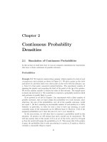
Figure 2.1 Pythagoras’ Theorem
is called the hypotenuse. Pythagoras’ Theorem is illustrated in Figure 2.1.
The ﬁgure shows a right-angled triangle, ABC, with hypotenuse AC, and two
other sides, AB and BC, of lengths x
1
and x
2
respectively. The squares on
each of the three sides of the triangle are drawn, and the area of the square
on the hypotenuse is shown as x
2
1

+ x
2
2
, in accordance with the theorem.
A beautiful proof of Pythagoras’ Theorem, not often found in geometry texts,
is shown in Figure 2.2. Two squares of equal area are drawn. Each square
contains four copies of the same right-angled triangle. The square on the left
also contains the squares on the two shorter sides of the triangle, while the

.
.
.
.
.
.
.
.
.
.
.
.
.
.
.
.
.
.
.
.
.

.
.
.
.
.
.
.
.
.
.
.
.
.
.
.
.
.
.
.
.
.
.
.
.
.
.
.
.
.
.

.
.
.
.
.

.
.
.
.
.
.
.
.
.
.
.
.
.
.
.
.
.
.
.
.
.
.
.
.

.
.
.
.
.
.
.
.
.
.
.
.
.
.
.
.
.
.
.
.
.
.
.
.
.
.
.
.
.
.

.
.
.

.
.
.
.
.
.
.
.
.
.
.
.
.
.
.
.
.
.
.
.
.
.
.
.
.
.

.
.
.
.
.
.
.
.
.
.
.
.
.
.
.
.
.
.
.
.
.
.
.
.
.
.
.
.
.
.

.
.
.
.
.
.
.
.
.
.
.
.
.
.
.
.
.
.
.
.
.
.
.

.
.
.
.
.
.

.
.
.
.
.
.
.
.
.
.
.
.
.
.
.
.
.
.
.
.
.
.
.
.
.
.
.
.
.
.

.

.
.
.
.
.
.
.
.
.
.
.
.
.
.
.
.
.
.
.
.
.
.
.
.
.
.
.
.

.
.
.
.
.
.
.
.
.
.
.
.
.
.
.
.
.
.
.
.
.
.
.
.
.
.
.
.
.
.

.
.
.
.
.
.
.
.
.
.
.
.
.
.
.
.
.
.
.
.
.
.
.
x
2
1
x
2
2

.
.
.
.
.
.
.
.
.
.
.
.
.
.
.
.
.
.
.
.
.
.
.
.
.
.
.
.
.
.

.
.
.
.
.
.
.
.
.
.
.
.
.
.
.
.
.
.
.
.
.
.
.
.
.
.

.
.
.

.
.
.
.
.
.
.
.
.
.
.
.
.
.
.
.
.
.
.
.
.
.
.
.
.
.
.
.
.
.

.
.
.
.
.
.
.
.
.
.
.
.
.
.
.
.
.
.
.
.
.
.
.
. .
.
.
.
.
.
.

.
.
.
.
.
.
.
.
.
.
.
.
.
.
.
.
.
.
.
.
.
.
.
.
.
.
.
.
.
.

.
.
.
.
.
.
.
.
.
.
.
.
.
.
.
.
.
.

.
.
.
.
.
.
.
.
.
.
.

.
.
.
.
.
.
.
.
.
.
.
.
.
.
.
.
.
.
.
.
.
.
.
.
.
.
.
.
.
.

.
.
.
.
.
.
.
.
.

.
.
.
.
.
.
.
.
.
.
.
.
.
.
.
.
.
.
.
.

.
.
.
.
.
.
.
.
.
.
.
.
.
.
.
.
.
.
.
.
.
.
.
.
.
.
.
.
.
.

.
.
.
.
.
x
2
1
+ x
2
2
Figure 2.2 Proof of Pythagoras’ Theorem
Copyright
c
 1999, Russell Davidson and James G. MacKinnon
46 The Geometry of Linear Regression

.
.
.
.
.
.
.
.
.
.
.
.
.

.
.
.
.
.
.
.
.
.
.
.
.
.
.
.
.
.
.
.
.
.
.
.
.
.
.
.
.
.
.

.
.
.
.
.
.
.
.
.
.
.
.
.
.
.
.
.
.
.

.
.
.
.
.
.
.
.
.
.

.
.
.
.
.
.
.
.
.
.
.
.
.
.
.
.
.
.
.
.
.
.
.
.
.
.
.
.
.
.

.
.
.
.
.
.
.
.
.
.
.
.
.
.
.
.

.
.
.
.
.
.
.
.
.
.
.
.
.

.
.
.
.
.
.
.
.
.
.
.
.
.
.
.
.
.
.
.
.
.
.
.
.
.
.
.
.
.
.

.
.
.
.
.
.
.
.
.
.
.
.
.
.
.
.
.
.
.
.
.

x
1
x
2
x
O
A
B

Figure 2.3 A vector x in E
2
square on the right contains the square on the hypotenuse. The theorem
follows at once.
Any vector x ∈ E
2
has two components, usually denoted as x
1
and x
2
. These
two components can be interpreted as the Cartesian coordinates of the vec-
tor in the plane. The situation is illustrated in Figure 2.3. With O as the
origin of the coordinates, a right-angled triangle is formed by the lines OA,
AB, and OB. The length of the horizontal side of the triangle, OA, is the
horizontal coordinate x
1
. The length of the vertical side, AB, is the vertical
coordinate x
2
. Thus the point B has Cartesian coordinates (x
1
, x
2
). The vec-
tor x itself is usually represented as the hypotenuse of the triangle, OB, that
is, the directed line (depicted as an arrow) joining the origin to the point B,
with coordinates (x
1
, x

2
). By Pythagoras’ Theorem, the length of the vector
x, the hypotenuse of the triangle, is (x
2
1
+x
2
2
)
1/2
. This is what (2.03) becomes
for the special case n = 2.
Vector Geometry in Two Dimensions
Let x and y be two vectors in E
2
, with components (x
1
, x
2
) and ( y
1
, y
2
),
respectively. Then, by the rules of matrix addition, the components of x + y
are (x
1
+ y
1
, x

2
+ y
2
). Figure 2.4 shows how the addition of x and y can
be performed geometrically in two diﬀerent ways. The vector x is drawn as
the directed line segment, or arrow, from the origin O to the point A with
coordinates (x
1
, x
2
). The vector y can be drawn similarly and represented
by the arrow OB. However, we could also draw y starting, not at O, but at
the point reached after drawing x, namely A. The arrow AC has the same
length and direction as OB, and we will see in general that arrows with the
same length and direction can be taken to represent the same vector. It is
clear by construction that the coordinates of C are (x
1
+ y
1
, x
2
+ y
2
), that is,
the coordinates of x + y. Thus the sum x + y is represented geometrically by
the arrow OC.
Copyright
c
 1999, Russell Davidson and James G. MacKinnon
2.2 The Geometry of Vector Spaces 47

.
.
.
.
.
.
.
.
.
.
.
.
.
.
.
.
.
.
.
.
.
.
.
.
.
.
.
.
.

.
.
.
.
.
.
.
.
.
.
.
.
.
.
.
.
.
.
.
.
.
.
.
.
.
.
.
.
.
.

.
.
.
.
.

.
.
.
.
.
.
.
.
.
.
.
.
.
.
.
.
.
.
.
.
.
.
.
.

.
.
.
.
.
.
.
.
.
.
.
.
.
.
.
.
.
.
.
.
.
.
.
.
.
.
.
.
.
.

.
.
.
.
.
.
.
.
.
.
.
.
.
.
.
.
.
.
.
.
.
.
.
.
.

.
.
.
.

.
.
.
.
.
.
.
.
.
.
.
.
.
.
.
.
.
.
.
.
.
.
.
.
.
.
.
.
.
.

.
.
.
.
.
.
.
.
.
.
.
.
.
.
.
.
.
.
.
.
.
.

.
.
.
.
.
.
.

.
.
.
.
.
.
.
.
.
.
.
.
.
.
.
.
.
.
.
.
.
.
.
.
.
.
.
.
.
.

.
.
.
.
.
.
.
.
.
.
.
.
.

.
.
.
.
.
.
.
.
.
.
.
.
.
.
.
.

.
.
.
.
.
.
.
.
.
.
.
.
.
.
.
.
.
.
.
.
.
.
.
.
.
.
.
.
.
.

.
.
.
.
.
.

.
.
.
.
.
.
.
.
.
.
.
.
.
.
.
.
.
.
.
.
.
.
.

.
.
.
.
.
.
.
.
.
.
.
.
.
.
.
.
.
.
.
.
.
.
.
.
.
.
.
.
.
.

.
.
.
.
.
.
.
.
.
.
.
.
.
.
.
.
.
.
.
.
.
.
.
.
.

O
A
C
B

x
x
y
x + y
y
x
1
y
1
x
2
y
2
Figure 2.4 Addition of vectors
The classical way of adding vectors geometrically is to form a parallelogram
using the line segments OA and OB that represent the two vectors as adjacent
sides of the parallelogram. The sum of the two vectors is then the diagonal
through O of the resulting parallelogram. It is easy to see that this classical
method also gives the result that the sum of the two vectors is represented
by the arrow OC, since the ﬁgure OACB is just the parallelogram required
by the construction, and OC is its diagonal through O. The parallelogram
construction also shows clearly that vector addition is commutative, since
y + x is represented by OB, for y, followed by BC, for x. The end result is
once more OC.
Multiplying a vector by a scalar is also very easy to represent geometrically.
If a vector x with components (x
1
, x
2
) is multiplied by a scalar α, then αx

has components (α x
1
, αx
2
). This is depicted in Figure 2.5, where α = 2. The
line segments OA and OB represent x and αx, respectively. It is clear that
even if we move αx so that it starts somewhere other than O, as with CD
in the ﬁgure, the vectors x and αx are always parallel. If α were negative,
then αx would simply point in the opposite direction. Thus, for α = −2, αx
would be represented by DC, rather than CD.
Another property of multiplication by a scalar is clear from Figure 2.5. By
direct calculation,
αx = αx, αx
1/2
= |α|(x

x)
1/2
= |α|x. (2.04)
Since α = 2, OB and CD in the ﬁgure are twice as long as OA.
Copyright
c
 1999, Russell Davidson and James G. MacKinnon
48 The Geometry of Linear Regression
.
.
.
.
.
.

.
.
.
.
.
.
.
.
.
.
.
.
.
.
.
.
.
.
.
.
.
.
.
.
.
.
.
.
.
.

.
.
.
.
.
.
.
.
.
.
.
.
.
.
.
.
.
.
.
.
.
.
.

.
.
.
.
.
.

.
.
.
.
.
.
.
.
.
.
.
.
.
.
.
.

.
.
.

.
.
.
.

.
.
.
.

.
.
.
.
.
.
.
.
.
.
.
.
.
.
.
.
.
.
.
.
.
.
.
.
.
.
.
.
.

.
.
.
.
.
.
.
.
.
.
.
.
.
.
.
.
.
.
.
.
.
.
.
.
.
.
.
.
.
.

.
.
.
.

.
.
.
.
.
.
.
.
.
.
.
.
.
.
.
.
.
.
.
.
.
.

.
.

.
.

.
.
.
.

.
.
.
.

.
.
.
.
.
.
.
.
.
.
.
.
.
.
.
.
.

.
.
.
.
.
.
.
.
.
.
.
.
.
.
.
.
.
.
.
.
.
.
.
.
.
.
.
.
.
.

.
.
.
.
.
.
.
.
.
.
.
.
.
.
.

.
.
.
.
.
.
.
.
.
.
.
.
.
.

.
.
.
.
.
.
.
.
.
.

.
.
.
.

.
.
.

.
.
.
.

.
.
O
A
•

B
C
D
x
αx
Figure 2.5 Multiplication by a scalar
The Geometry of Scalar Products
The scalar product of two vectors x and y, whether in E
2
or E
n
, can be
expressed geometrically in terms of the lengths of the two vectors and the
angle between them, and this result will turn out to be very useful. In the
case of E
2
, it is natural to think of the angle between two vectors as the angle
between the two line segments that represent them. As we will now show, it
is also quite easy to deﬁne the angle between two vectors in E
n
.
If the angle between two vectors is 0, they must be parallel. The vector y is
parallel to the vector x if y = αx for some suitable α. In that event,
x, y = x, αx = αx

x = αx
2
.
From (2.04), we know that y = |α|x, and so, if α > 0, it follows that
x, y = x y. (2.05)

Of course, this result is true only if x and y are parallel and point in the same
direction (rather than in opposite directions).
For simplicity, consider initially two vectors, w and z, both of length 1, and
let θ denote the angle between them. This is illustrated in Figure 2.6. Suppose
that the ﬁrst vector, w, has coordinates (1, 0). It is therefore represented by
a horizontal line of length 1 in the ﬁgure. Supp ose that the second vector, z,
is also of length 1, that is, z = 1. Then, by elementary trigonometry, the
coordinates of z must be (cos θ, sin θ). To show this, note ﬁrst that, if so,
z
2
= cos
2
θ + sin
2
θ = 1, (2.06)
as required. Next, consider the right-angled triangle OAB, in which the hy-
potenuse OB represents z and is of length 1, by (2.06). The length of the
side AB opposite O is sin θ, the vertical coordinate of z. Then the sine of
Copyright
c
 1999, Russell Davidson and James G. MacKinnon
2.2 The Geometry of Vector Spaces 49

.
.
.
.
.
.
.

.
.
.
.
.
.
.
.
.
.
.
.
.
.
.
.
.
.
.
.
.
.
.
.
.
.
.
.
.
.

.
.
.
.
.
.
.
.
.
.
.
.
.
.
.
.
.
.
.
.
.

.
.
.
.
.
.
.
.

.
.
.
.
.
.
.
.
.
.
.
.
.
.
.
.
.
.
.
.
.
.
.
.
.
.
.
.
.
.

.
.
.
.
.
.
.
.
.
.
.
.
.
.
.

.
.
.
.
.
.
.
.
.
.
.
.
.
.

.
.
.
.
.
.
.
.
.
.
.
.
.
.
.
.
.
.
.
.
.
.
.
.
.
.
.
.
.
.

.
.
.
.
.
.
.
.
.
.
.
.
.
.
.
.
.
.
.
.
.
.
.
.
.
.
.
O
A
B

w
z
θ
Figure 2.6 The angle between two vectors
the angle BOA is given, by the usual trigonometric rule, by the ratio of the
length of the opposite side AB to that of the hypotenuse OB. This ratio is
sin θ/1 = sin θ, and so the angle BOA is indeed equal to θ.
Now let us compute the scalar product of w and z. It is
w, z = w

z = w
1
z
1
+ w
2
z
2
= z
1
= cos θ,
because w
1
= 1 and w
2
= 0. This result holds for vectors w and z of length 1.
More generally, let x = αw and y = γz, for positive scalars α and γ. Then
x = α and y = γ. Thus we have
x, y = x


y = αγw

z = αγw, z.
Because x is parallel to w, and y is parallel to z, the angle between x and y
is the same as that between w and z, namely θ. Therefore,
x, y = x y cos θ. (2.07)
This is the general expression, in geometrical terms, for the scalar product of
two vectors. It is true in E
n
just as it is in E
2
, although we have not proved
this. In fact, we have not quite proved (2.07) even for the two-dimensional
case, because we made the simplifying assumption that the direction of x
and w is horizontal. In Exercise 2.1, we ask the reader to provide a more
complete proof.
The cosine of the angle between two vectors provides a natural way to measure
how close two vectors are in terms of their directions. Recall that cos θ varies
between −1 and 1; if we measure angles in radians, cos 0 = 1, cos π / 2 = 0,
and cos π = −1. Thus cos θ will be 1 for vectors that are parallel, 0 for vectors
that are at right angles to each other, and −1 for vectors that point in directly
Copyright
c
 1999, Russell Davidson and James G. MacKinnon
50 The Geometry of Linear Regression
opposite directions. If the angle θ between the vectors x and y is a right angle,
its cosine is 0, and so, from (2.07), the scalar product x, y is 0. Conversely,
if x, y = 0, then cos θ = 0 unless x or y is a zero vector. If cos θ = 0, it
follows that θ = π/2. Thus, if two nonzero vectors have a zero scalar product,
they are at right angles. Such vectors are often said to be orthogonal, or,

less commonly, perpendicular. This deﬁnition implies that the zero vector is
orthogonal to everything.
Since the cosine function can take on values only between −1 and 1, a conse-
quence of (2.07) is that
|x

y| ≤ x y. (2.08)
This result, which is called the Cauchy-Schwartz inequality, says that the
inner product of x and y can never be greater than the length of the vector x
times the length of the vector y. Only if x and y are parallel does the
inequality in (2.08) become the equality (2.05). Readers are asked to prove
this result in Exercise 2.2.
Subspaces of Euclidean Space
For arbitrary positive integers n, the elements of an n vector can be thought
of as the coordinates of a point in E
n
. In particular, in the regression model
(2.01), the regressand y and each column of the matrix of regressors X can be
thought of as vectors in E
n
. This makes it possible to represent a relationship
like (2.01) geometrically.
It is obviously impossible to represent all n dimensions of E
n
physically
when n > 3. For the pages of a book, even three dimensions can be too many,
although a proper use of perspective drawings can allow three dimensions to
be shown. Fortunately, we can represent (2.01) without needing to draw in
n dimensions. The key to this is that there are only three vectors in (2.01):
y, Xβ, and u. Since only two vectors, Xβ and u, appear on the right-hand

side of (2.01), only two dimensions are needed to represent it. Because y is
equal to Xβ + u, these two dimensions suﬃce for y as well.
To see how this works, we need the concept of a subspace of a Euclidean
space E
n
. Normally, such a subspace will have a dimension lower than n. The
easiest way to deﬁne a subspace of E
n
is in terms of a set of basis vectors. A
subspace that is of particular interest to us is the one for which the columns
of X provide the basis vectors. We may denote the k columns of X as x
1
,
x
2
, . . . x
k
. Then the subspace associated with these k basis vectors will be
denoted by S(X) or S(x
1
, . . . , x
k
). The basis vectors are said to span this
subspace, which will in general be a k dimensional subspace.
The subspace S(x
1
, . . . , x
k
) consists of every vector that can be formed as a
linear combination of the x

i
, i = 1, . . . , k. Formally, it is deﬁned as
S(x
1
, . . . , x
k
) ≡

z ∈ E
n



z =
k

i=1
b
i
x
i
, b
i
∈ R

. (2.09)
Copyright
c
 1999, Russell Davidson and James G. MacKinnon
2.2 The Geometry of Vector Spaces 51

.
.
.
.
.
.
.
.
.
.
.
.
.
.
.
.
.
.
.
.
.
.
.
.
.
.
.
.
.
.

.
.
.
.
.
.
.
.
.
.
.
.
.
.
.
.
.
.

.
.
.
.
.
.
.
.
.
.
.

.
.
.
.
.
.
.
.
.
.
.
.
.
.
.
.
.
.
.
.
.
.
.
.
.
.
.
.
.
.

.
.
.
.
.
.
.
.
.
.
.
.
.
.
.
.
.
.
.
.
.
.
.
.

.
.
.
.
.

.
.
.
.
.
.
.
.
.
.
.
.
.
.
.
.
.
.
.
.
.
.
.
.
.
.
O
x
S(X)
S

⊥
(X)
Figure 2.7 The spaces S(X) and S
⊥
(X)
The subspace deﬁned in (2.09) is called the subspace spanned by the x
i
,
i = 1, . . . , k, or the column space of X; less formally, it may simply be referred
to as the span of X, or the span of the x
i
.
The orthogonal complement of S(X) in E
n
, which is denoted S
⊥
(X), is the
set of all vectors w in E
n
that are orthogonal to everything in S(X). This
means that, for every z in S(X), w, z = w

z = 0. Formally,
S
⊥
(X) ≡

w ∈ E
n
| w


z = 0 for all z ∈ S(X)

.
If the dimension of S(X) is k, then the dimension of S
⊥
(X) is n − k.
Figure 2.7 illustrates the concepts of a subspace and its orthogonal comple-
ment for the simplest case, in which n = 2 and k = 1. The matrix X has
only one column in this case, and it is therefore represented in the ﬁgure by a
single vector, denoted x. As a consequence, S(X) is 1 dimensional, and, since
n = 2, S
⊥
(X) is also 1 dimensional. Notice that S(X) and S
⊥
(X) would be
the same if x were any vector, except for the origin, parallel to the straight
line that represents S(X).
Now let us return to E
n
. Suppose, to b egin with, that k = 2. We have two
vectors, x
1
and x
2
, which span a subspace of, at most, two dimensions. It
is always possible to represent vectors in a 2 dimensional space on a piece of
paper, whether that space is E
2
itself or, as in this case, the 2 dimensional

subspace of E
n
spanned by the vectors x
1
and x
2
. To represent the ﬁrst
vector, x
1
, we choose an origin and a direction, b oth of which are entirely
arbitrary, and draw an arrow of length x
1
 in that direction. Suppose that
the origin is the point O in Figure 2.8, and that the direction is the horizontal
direction in the plane of the page. Then an arrow to represent x
1
can be
drawn as shown in the ﬁgure. For x
2
, we compute its length, x
2
, and the
angle, θ, that it makes with x
1
. Suppose for now that θ = 0. Then we choose
Copyright
c
 1999, Russell Davidson and James G. MacKinnon
52 The Geometry of Linear Regression

.
.
.
.
.
.
.
.
.
.
.
.
.
.
.
.
.
.
.
.
.
.
.
.
.
.
.
.
.
.

.
.
.
.
.
.
.
.
.
.
.
.
.

.
.
.
.
.
.
.
.
.
.
.
.
.
.
.
.

.
.
.
.
.
.
.
.
.
.
.
.
.
.
.
.
.
.
.
.
.
.
.
.
.
.
.
.
.
.

.
.
.
.
.
.
.
.
.

.
.
.
.
.
.
.
.
.
.
.
.
.
.
.
.
.
.
.
.

.
.
.
.
.
.
.
.
.
.
.
.
.
.
.
.
.
.
.
.
.
.
.
.
.
.
.
.
.
.

.
.
.
.
.

.
.
.
.
.
.
.
.
.
.
.
.
.
.
.
.
.
.
.
.
.
.
.
.

.
.
.
.
.
.
.
.
.
.
.
.
.
.
.
.
.
.
.
.
.
.
.
.
.
.
.
.
.
.

.
.
.
.
.
.
.

.
.
.
.
.
.
.
.
.
.
.
.
.
.
.
.
.
.
.
.
.
.

.
.
.

.
.
.
.
.
.

.
.
.
.
.
.
.
.
.
.
.
.
.
.
.

.
.
.
.
.
.
.
.
.
.
.
.
.
.
.
.
.
.
.
.
.
.
.
.
.
.
.
.
.
.

.
.
.
.
.

.
.
.
.
.
.
.
.
.
.
.
.
.
.
.
.
.
.
.
.
.
.
.
.

.
.
.
.
.
.
.
.
.
.
.
.
.
.
.
.
.
.
.
.
.
.
.
.
.
.
.
.
.
.

.
.
O
x
1
x
2
b
1
x
1
b
2
x
2
b
1
x
1
+ b
2
x
2
θ
Figure 2.8 A 2-dimensional subspace
as our second dimension the vertical direction in the plane of the page, with
the result that we can draw an arrow for x
2
, as shown.
Any vector in S(x

1
, x
2
) can be drawn in the plane of Figure 2.8. Consider,
for instance, the linear combination of x
1
and x
2
given by the expression
z ≡ b
1
x
1
+ b
2
x
2
. We could draw the vector z by computing its length and
the angle that it makes with x
1
. Alternatively, we could apply the rules for
adding vectors geometrically that were illustrated in Figure 2.4 to the vectors
b
1
x
1
and b
2
x
2

. This is illustrated in the ﬁgure for the case in which b
1
=
2
/
3
and b
2
=
1
/
2
.
In precisely the same way, we can represent any three vectors by arrows in
3 dimensional space, but we leave this task to the reader. It will be easier to
appreciate the renderings of vectors in three dimensions in perspective that
appear later on if one has already tried to draw 3 dimensional pictures, or
even to model relationships in three dimensions with the help of a computer.
We can ﬁnally represent the regression model (2.01) geometrically. This is
done in Figure 2.9. The horizontal direction is chosen for the vector Xβ, and
then the other two vectors y and u are shown in the plane of the page. It
is clear that, by construction, y = Xβ + u. Notice that u, the error vector,
is not orthogonal to Xβ. The ﬁgure contains no reference to any system of
axes, because there would be n of them, and we would not be able to avoid
needing n dimensions to treat them all.
Linear Independence
In order to deﬁne the OLS estimator by the formula (1.46), it is necessary
to assume that the k × k square matrix X

X is invertible, or nonsingular.

Equivalently, as we saw in Section 1.4, we may say that X

X has full rank.
This condition is equivalent to the condition that the columns of X should be
linearly independent. This is a very important concept for econometrics. Note
that the meaning of linear independence is quite diﬀerent from the meaning
Copyright
c
 1999, Russell Davidson and James G. MacKinnon
2.2 The Geometry of Vector Spaces 53

.
.
.
.
.
.
.
.
.
.
.
.
.
.
.
.
.
.
.

.
.
.
.
.
.
.
.
.
.
.
.
.
.
.
.
.
.
.
.
.
.
.
.
.
.
.
.
.
.

.
.
.
.
.
.
.
.
.
.
.
.
.
.
.
.
.
.
.
.
.
.
.
.
.
.

.
.
.

.
.
.
.
.
.
.
.
.
.
.
.
.
.
.
.
.
.
.
.
.
.
.
.
.
.
.
.
.
.

O
Xβ
u
y
Figure 2.9 The geometry of the linear regression model
of statistical independence, which we discussed in Section 1.2. It is important
not to confuse these two concepts.
The vectors x
1
through x
k
are said to be linearly dependent if we can write
one of them as a linear combination of the others. In other words, there is a
vector x
j
, 1 ≤ j ≤ k , and coeﬃcients c
i
such that
x
j
=

i=j
c
i
x
i
. (2.10)
Another, equivalent, deﬁnition is that there exist coeﬃcients b
i

, at least one
of which is nonzero, such that
k

i=1
b
i
x
i
= 0. (2.11)
Recall that 0 denotes the zero vector, every component of which is 0. It is
clear from the deﬁnition (2.11) that, if any of the x
i
is itself equal to the zero
vector, then the x
i
are linearly dependent. If x
j
= 0, for example, then (2.11)
will be satisﬁed if we make b
j
nonzero and set b
i
= 0 for all i = j.
If the vectors x
i
, i = 1, . . . , k, are the columns of an n × k matrix X, then
another way of writing (2.11) is
Xb = 0, (2.12)
where b is a k vector with typical element b

i
. In order to see that (2.11)
and (2.12) are equivalent, it is enough to check that the typical elements of
the two left-hand sides are the same; see Exercise 2.5. The set of vectors
x
i
, i = 1, . . . , k, is linearly independent if it is not linearly dependent, that
is, if there are no coeﬃcients c
i
such that (2.10) is true, or (equivalently) no
Copyright
c
 1999, Russell Davidson and James G. MacKinnon
54 The Geometry of Linear Regression
coeﬃcients b
i
such that (2.11) is true, or (equivalently, once more) no vector
b such that (2.12) is true.
It is easy to show that if the columns of X are linearly dependent, the matrix
X

X is not invertible. Premultiplying (2.12) by X

yields
X

Xb = 0. (2.13)
Thus, if the columns of X are linearly dependent, there is a nonzero k vector
b which is annihilated by X


X. The existence of such a vector b means that
X

X cannot be inverted. To see this, consider any vector a, and suppose
that
X

Xa = c.
If X

X could be inverted, then we could premultiply the above equation by
(X

X)
−1
to obtain
(X

X)
−1
c = a. (2.14)
However, (2.13) also allows us to write
X

X(a + b) = c,
which would give
(X

X)
−1

c = a + b. (2.15)
But (2.14) and (2.15) cannot both be true, and so (X

X)
−1
cannot exist.
Thus a necessary condition for the existence of (X

X)
−1
is that the columns
of X should be linearly independent. With a little more work, it can be shown
that this condition is also suﬃcient, and so, if the regressors x
1
, . . . , x
k
are
linearly independent, X

X is invertible.
If the k columns of X are not linearly independent, then they will span a
subspace of dimension less than k, say k

, where k

is the largest number of
columns of X that are linearly independent of each other. The number k

is
called the rank of X. Look again at Figure 2.8, and imagine that the angle θ

between x
1
and x
2
tends to zero. If θ = 0, then x
1
and x
2
are parallel, and we
can write x
1
= αx
2
, for some scalar α. But this means that x
1
−αx
2
= 0, and
so a relation of the form (2.11) holds between x
1
and x
2
, which are therefore
linearly dependent. In the ﬁgure, if x
1
and x
2
are parallel, then only one
dimension is used, and there is no need for the second dimension in the plane
of the page. Thus, in this case, k = 2 and k


= 1.
When the dimension of S(X) is k

< k, S(X) will be identical to S(X

), where
X

is an n × k

matrix consisting of any k

linearly indep endent columns of
X. For example, consider the following X matrix, which is 5 × 3:





1 0 1
1 4 0
1 0 1
1 4 0
1 0 1






. (2.16)
Copyright
c
 1999, Russell Davidson and James G. MacKinnon
2.3 The Geometry of OLS Estimation 55
The columns of this matrix are not linearly independent, since
x
1
= .25x
2
+ x
3
.
However, any two of the columns are linearly independent, and so
S(X) = S(x
1
, x
2
) = S(x
1
, x
3
) = S(x
2
, x
3
);
see Exercise 2.8. For the remainder of this chapter, unless the contrary is
explicitly assumed, we will assume that the columns of any regressor matrix
X are linearly independent.

2.3 The Geometry of OLS Estimation
We studied the geometry of vector spaces in the last section because the nu-
merical properties of OLS estimates are easily understood in terms of that
geometry. The geometrical interpretation of OLS estimation, that is, MM es-
timation of linear regression models, is simple and intuitive. In many cases,
it entirely does away with the need for algebraic proofs.
As we saw in the last section, any point in a subspace S(X), where X is an
n ×k matrix, can be represented as a linear combination of the columns of X.
We can partition X in terms of its columns explicitly, as follows:
X = [ x
1
x
2
· · · x
k
] .
In order to compute the matrix product Xβ in terms of this partitioning, we
need to partition the vector β by its rows. Since β has only one column, the
elements of the partitioned vector are just the individual elements of β. Thus
we ﬁnd that
Xβ = [ x
1
x
2
· · · x
k
]





β
1
β
2
.
.
.
β
k




= x
1
β
1
+ x
2
β
2
+ . . . + x
k
β
k
=
k

i=1

β
i
x
i
,
which is just a linear combination of the columns of X. In fact, it is clear
from the deﬁnition (2.09) that any linear combination of the columns of X,
and thus any element of the subspace S(X) = S(x
1
, . . . , x
k
), can be written
as Xβ for some β. The speciﬁc linear combination (2.09) is constructed by
using β = [b
1
.
.
.
.
. . .
.
.
.
.
b
k
]. Thus every n vector Xβ belongs to S(X), which
is, in general, a k dimensional subspace of E
n
. In particular, the vector X

ˆ
β
constructed using the OLS estimator
ˆ
β belongs to this subspace.
The estimator
ˆ
β was obtained by solving the equations (1.48), which we
rewrite here for easy reference:
X

(y − X
ˆ
β) = 0. (1.48)
Copyright
c
 1999, Russell Davidson and James G. MacKinnon
56 The Geometry of Linear Regression

.
.
.
.
.
.
.
.
.
.
.

.
.
.
.
.
.
.
.
.
.
.
.
.
.
.
.
.
.
.
.
.
.
.
.
.
.
.
.
.
.

.
.
.
.
.
.
.
.
.
.
.
.
.
.
.
.
.
.
.
.
.
.

.
.
.
.
.
.
.

.
.
.
.
.
.
.
.
.
.
.
.
.
.
.
.
.
.
.
.
.
.
.
.
.
.
.
.
.
.

.
.
.
.
.

.
.
.
.
.
.
.
.
.
.
.
.
.
.
.
.
.
.
.
.
.
.
.
.

.
.
.
.
.
.
.
.
.
.
.
.
.
.
.
.
.
.
.
.
.
.
.
.
.
.
.
.
.
.

.
.
.
.
.
.
.
.
.
.
.
.
.
.
.
.
.
.
.
.
.
.
.
.
.

.
.
.
.

.
.
.
.
.
.
.
.
.
.
.
.
.
.
.
.
.
.
.
.
.
.
.
.
.
.
.
.
.
.

.
.
.
.
.
.
.
.
.
.
.
.
.
.
.
.
O
y
ˆ
u
X
ˆ
β
θ
Figure 2.10 Residuals and ﬁtted values
These equations have a simple geometrical interpretation. Note ﬁrst that each
element of the left-hand side of (1.48) is a scalar product. By the rule for
selecting a single row of a matrix product (see Section 1.4), the i
th
element is

x
i

(y − X
ˆ
β) = x
i
, y − X
ˆ
β, (2.17)
since x
i
, the i
th
column of X, is the transpose of the i
th
row of X

. By (1.48),
the scalar product in (2.17) is zero, and so the vector y − X
ˆ
β is orthogonal to
all of the regressors, that is, all of the vectors x
i
that represent the explanatory
variables in the regression. For this reason, equations like (1.48) are often
referred to as orthogonality conditions.
Recall from Section 1.5 that the vector y − Xβ, treated as a function of β,
is called the vector of residuals. This vector may be written as u(β). We
are interested in u(

ˆ
β), the vector of residuals evaluated at
ˆ
β, which is often
called the vector of least squares residuals and is usually written simply as
ˆ
u.
We have just seen, in (2.17), that
ˆ
u is orthogonal to all the regressors. This
implies that
ˆ
u is in fact orthogonal to every vector in S(X), the span of the
regressors. To see this, remember that any element of S(X) can be written
as Xβ for some β, with the result that, by (1.48),
Xβ,
ˆ
u = (Xβ)

ˆ
u = β

X

ˆ
u = 0.
The vector X
ˆ
β is referred to as the vector of ﬁtted values. Clearly, it lies
in S(X), and, consequently, it must be orthogonal to

ˆ
u. Figure 2.10 is similar
to Figure 2.9, but it shows the vector of least squares residuals
ˆ
u and the
vector of ﬁtted values X
ˆ
β instead of u and Xβ. The key feature of this
ﬁgure, which is a consequence of the orthogonality conditions (1.48), is that
the vector
ˆ
u makes a right angle with the vector X
ˆ
β.
Some things about the orthogonality conditions (1.48) are clearer if we add
a third dimension to the picture. Accordingly, in panel a) of Figure 2.11,
Copyright
c
 1999, Russell Davidson and James G. MacKinnon
2.3 The Geometry of OLS Estimation 57

.
.
.
.
.
.
.
.
.

.
.
.
.
.
.
.
.
.
.
.
.
.
.
.
.
.
.
.
.
.
.
.
.
.
.
.
.
.
.

.
.
.
.
.
.
.
.
.
.
.
.
.
.
.
.
.
.
.
.
.
.
.
.
.
.
.

.
.

.
.
.
.
.
.
.
.
.
.
.
.
.
.
.
.
.
.
.
.
.
.
.
.
.
.
.
.
.
.

.
.
.
.
.
.
.
.
.
.
.
.
.
.
.
.
.
.
.
.
.
.

.
.
.
.
.
.
.

.
.
.
.
.
.
.
.
.
.
.
.
.
.
.
.
.
.
.
.
.
.
.
.
.
.
.
.
.
.

.
.
.
.
.
.
.
.
.
.
.
.
.
.
.

.
.
.
.
.
.
.
.
.
.
.
.
.
.

.
.
.
.
.
.
.
.
.
.
.
.
.
.
.
.
.
.
.
.
.
.
.
.
.
.
.
.
.
.

.
.
.
.
.
.
.
.
.
.
.
.
.
.
.
.
.
.
.
.
.
.
.
.
.
.

.
.
.

.
.
.
.
.
.
.
.
.
.
.
.
.
.
.
.
.
.
.
.
.
.
.
.
.
.
.
.
.
.

.

.
.
.
.
.
.
.
.
.
.
.
.
.
.
.
.
.
.
.
.
.
.
.
.
.
.
.
.

.
.
.
.
.
.
.
.
.
.
.
.
.
.
.
.
.
.
.
.
.
.
.
.
.
.
.
.
.
.

x
1
x
2
y
X
ˆ
β
ˆ
u
S(x
1
, x
2
)
O
A
B
θ
a) y projected on two regressors

.
.
.
.
.
.
.
.
.

.
.
.
.
.
.
.
.
.
.
.
.
.
.
.
.
.
.
.
.
.
.
.
.
.
.
.
.
.
.

.
.
.
.
.

.
.
.
.
.
.
.
.
.
.
.
.
.
.
.
.
.
.
.
.
.
.
.
.

.
.
.
.
.
.
.
.
.
.
.
.
.
.
.
.
.
.
.
.
.
.
.
.
.
.
.
.
.
.

.
.
.

.
.
.
.
.
.
.
.
.
.
.
.
.
.
.
.
.
.
.
.
.
.
.
.
.
.

.
.
.
.
.
.
.
.
.
.
.
.
.
.
.
.
.
.
.
.
.
.
.
.
.
.
.
.
.
.

.
.
.
.
.
.
.
.
.
.
.
.
.
.
.
.
.
.

.
.
.
.
.
.
.
.
.
.
.

.
.
.
.
.
.
.
.
.
.
.
.
.
.
.
.
.
.
.
.
.
.
.
.
.
.
.
.
.
.

.
.
.
.
.
.
.
.
.
.
.
.
O
x
1
x
2
X
ˆ
β
A
ˆ
β
1
x
1
ˆ
β
2
x

2
b) The span S(x
1
, x
2
) of the regressors
.
.
.
.
.
.
.
.
.
.
.
.
.
.
.
.
.
.
.
.
.
.
.
.

.
.
.
.
.
.
.
.
.
.
.
.
.
.
.
.
.
.
.
.
.
.
.
.
.
.
.
.
.
.

.
.
.
.
.
.
.
.
.
.
.
.
.
.
.

.
.
.
.
.
.
.
.
.
.
.
.
.
.

.
.
.
.
.
.
.
.
.
.
.
.
.
.
.
.
.
.
.
.
.
.
.
.
.
.
.
.
.
.

.
.
.
.
.
.
.
.
.
.
.
.
.
.
.
.
.
.
.
.
.
.
.
.

.
.
.
.
.

.
.
.
.
.
.
.
.
.
.
.
.
.
.
.
.
.
.
.
.
.
.
.
.
.
.
.
.
.
.

.
.
.
.
.
.
.
.
.
.
.
.
.
.
.
.
.
.
.
.
.
.

.
.
.
.
.
.
.

.
.
.
.
.
.
.
.
.
.
.
.
.
.
.
.
.
.
.
.
.
.
.
.
.
.
.
.
.
.

.
y
X
ˆ
β
ˆ
u
O A
B
θ
c) The vertical plane through y
Figure 2.11 Linear regression in three dimensions
we consider the case of two regressors, x
1
and x
2
, which together span the
horizontal plane labelled S(x
1
, x
2
), seen in perspective from slightly above
the plane. Although the perspective rendering of the ﬁgure does not make it
clear, both the lengths of x
1
and x
2
and the angle between them are totally
arbitrary, since they do not aﬀect S(x
1

, x
2
) at all. The vector y is intended
to be viewed as rising up out of the plane spanned by x
1
and x
2
.
In the 3 dimensional setup, it is clear that, if
ˆ
u is to be orthogonal to the
horizontal plane, it must itself be vertical. Thus it is obtained by “dropping
a perpendicular” from y to the horizontal plane. The least-squares inter-
pretation of the MM estimator
ˆ
β can now be seen to be a consequence of
simple geometry. The shortest distance from y to the horizontal plane is
obtained by descending vertically on to it, and the point in the horizontal
plane vertically below y, labeled A in the ﬁgure, is the closest point in the
plane to y. Thus 
ˆ
u minimizes u(β), the norm of u(β), with respect to β.
Copyright
c
 1999, Russell Davidson and James G. MacKinnon
58 The Geometry of Linear Regression
The squared norm, u(β)
2
, is just the sum of squared residuals, SSR(β);
see (1.49). Since minimizing the norm of u(β) is the same thing as minimiz-

ing the squared norm, it follows that
ˆ
β is the OLS estimator.
Panel b) of the ﬁgure shows the horizontal plane S(x
1
, x
2
) as a straightfor-
ward 2 dimensional picture, seen from directly above. The point A is the
point directly underneath y, and so, since y = X
ˆ
β +
ˆ
u by deﬁnition, the
vector represented by the line segment OA is the vector of ﬁtted values, X
ˆ
β.
Geometrically, it is much simpler to represent X
ˆ
β than to represent just the
vector
ˆ
β, because the latter lies in R
k
, a diﬀerent space from the space E
n
that contains the variables and all linear combinations of them. However, it is
easy to see that the information in panel b) does indeed determine
ˆ
β. Plainly,

X
ˆ
β can be decomposed in just one way as a linear combination of x
1
and x
2
,
as shown. The numerical value of
ˆ
β
1
can be computed as the ratio of the
length of the vector
ˆ
β
1
x
1
to that of x
1
, and similarly for
ˆ
β
2
.
In panel c) of Figure 2.11, we show the right-angled triangle that corresponds
to dropping a perpendicular from y, labelled in the same way as in panel a).
This triangle lies in the vertical plane that contains the vector y. We can see
that y is the hypotenuse of the triangle, the other two sides being X
ˆ

β and
ˆ
u.
Thus this panel corresponds to what we saw already in Figure 2.10. Since we
have a right-angled triangle, we can apply Pythagoras’ Theorem. It gives
y
2
= X
ˆ
β
2
+ 
ˆ
u
2
. (2.18)
If we write out the squared norms as scalar products, this becomes
y

y =
ˆ
β

X

X
ˆ
β + (y − X
ˆ
β)


(y − X
ˆ
β). (2.19)
In words, the total sum of squares, or TSS, is equal to the explained sum
of squares, or ESS, plus the sum of squared residuals, or SSR. This is a
fundamental property of OLS estimates, and it will prove to be very useful in
many contexts. Intuitively, it lets us break down the total variation (TSS) of
the dependent variable into the explained variation (ESS) and the unexplained
variation (SSR), unexplained because the residuals represent the aspects of y
about which we remain in ignorance.
Orthogonal Projections
When we estimate a linear regression model, we implicitly map the regressand
y into a vector of ﬁtted values X
ˆ
β and a vector of residuals
ˆ
u = y − X
ˆ
β.
Geometrically, these mappings are examples of orthogonal projections. A
projection is a mapping that takes each point of E
n
into a point in a subspace
of E
n
, while leaving all points in that subspace unchanged. Because of this,
the subspace is called the invariant subspace of the projection. An orthogonal
projection maps any point into the point of the subspace that is closest to it.
If a point is already in the invariant subspace, it is mapped into itself.

Copyright
c
 1999, Russell Davidson and James G. MacKinnon
2.3 The Geometry of OLS Estimation 59
The concept of an orthogonal projection formalizes the notion of “dropping
a perpendicular” that we used in the last subsection when discussing least
squares. Algebraically, an orthogonal projection on to a given subspace can
be performed by premultiplying the vector to be projected by a suitable pro-
jection matrix. In the case of OLS, the two projection matrices that yield the
vector of ﬁtted values and the vector of residuals, respectively, are
P
X
= X(X

X)
−1
X

, and
M
X
= I − P
X
= I − X(X

X)
−1
X

,

(2.20)
where I is the n × n identity matrix. To see this, recall (2.02), the formula
for the OLS estimates of β:
ˆ
β = (X

X)
−1
X

y.
From this, we see that
X
ˆ
β = X(X

X)
−1
X

y = P
X
y. (2.21)
Therefore, the ﬁrst projection matrix in (2.20), P
X
, projects on to S(X). For
any n vector y, P
X
y always lies in S(X), because
P

X
y = X

(X

X)
−1
X

y

.
Since this takes the form Xb for b =
ˆ
β, it is a linear combination of the
columns of X, and hence it belongs to S(X).
From (2.20), it is easy to show that P
X
X = X. Since any vector in S(X)
can be written as Xb for some b ∈ R
k
, we see that
P
X
Xb = Xb. (2.22)
We saw from (2.21) that the result of acting on any vector y ∈ E
n
with P
X
is

a vector in S(X). Thus the invariant subspace of the projection P
X
must be
contained in S(X). But, by (2.22), every vector in S(X) is mapped into itself
by P
X
. Therefore, the image of P
X
, which is a shorter name for its invariant
subspace, is precisely S(X).
It is clear from (2.21) that, when P
X
is applied to y, it yields the vector of
ﬁtted values. Similarly, when M
X
, the second of the two projection matrices
in (2.20), is applied to y, it yields the vector of residuals:
M
X
y =

I − X(X

X)
−1
X


y = y − P
X

y = y − X
ˆ
β =
ˆ
u.
The image of M
X
is S
⊥
(X), the orthogonal complement of the image of P
X
.
To see this, consider any vector w ∈ S
⊥
(X). It must satisfy the deﬁning condi-
tion X

w = 0. From the deﬁnition (2.20) of P
X
, this implies that P
X
w = 0,
Copyright
c
 1999, Russell Davidson and James G. MacKinnon
60 The Geometry of Linear Regression
the zero vector. Since M
X
= I − P
X

, we ﬁnd that M
X
w = w. Thus S
⊥
(X)
must be contained in the image of M
X
. Next, consider any vector in the
image of M
X
. It must take the form M
X
y, where y is some vector in E
n
.
From this, it will follow that M
X
y belongs to S
⊥
(X). Observe that
(M
X
y)

X = y

M
X
X, (2.23)
an equality that relies on the symmetry of M

X
. Then, from (2.20), we have
M
X
X = (I − P
X
)X = X − X = O, (2.24)
where O denotes a zero matrix, which in this case is n × k. The result (2.23)
says that any vector M
X
y in the image of M
X
is orthogonal to X, and thus
belongs to S
⊥
(X). We saw above that S
⊥
(X) was contained in the image
of M
X
, and so this image must coincide with S
⊥
(X). For obvious reasons,
the projection M
X
is sometimes called the projection oﬀ S(X).
For any matrix to represent a projection, it must be idempotent. An idem-
potent matrix is one that, when multiplied by itself, yields itself again. Thus,
P
X

P
X
= P
X
and M
X
M
X
= M
X
.
These results are easily proved by a little algebra directly from (2.20), but the
geometry of the situation makes them obvious. If we take any point, project
it on to S(X), and then project it on to S(X) again, the second projection
can have no eﬀect at all, because the point is already in S(X), and so it is
left unchanged. Since this implies that P
X
P
X
y = P
X
y for any vector y, it
must be the case that P
X
P
X
= P
X
, and similarly for M
X

.
Since, from (2.20),
P
X
+ M
X
= I, (2.25)
any vector y ∈ E
n
is equal to P
X
y + M
X
y. The pair of projections P
X
and
M
X
are said to be complementary projections, since the sum of P
X
y and
M
X
y restores the original vector y.
The fact that S(X) and S
⊥
(X) are orthogonal subspaces leads us to say that
the two projection matrices P
X
and M

X
deﬁne what is called an orthogonal
decomposition of E
n
, because the two vectors M
X
y and P
X
y lie in the two
orthogonal subspaces. Algebraically, the orthogonality depends on the fact
that P
X
and M
X
are symmetric matrices. To see this, we start from a
further important property of P
X
and M
X
, which is that
P
X
M
X
= O. (2.26)
This equation is true for any complementary pair of projections satisfy-
ing (2.25), whether or not they are symmetric; see Exercise 2.9. We may say
that P
X
and M

X
annihilate each other. Now consider any vector z ∈ S(X)
Copyright
c
 1999, Russell Davidson and James G. MacKinnon
2.3 The Geometry of OLS Estimation 61
and any other vector w ∈ S
⊥
(X). We have z = P
X
z and w = M
X
w. Thus
the scalar product of the two vectors is
P
X
z, M
X
w = z

P

X
M
X
w.
Since P
X
is symmetric, P


X
= P
X
, and so the above scalar product is zero
by (2.26). In general, however, if two complementary projection matrices are
not symmetric, the spaces they project on to are not orthogonal.
The projection matrix M
X
annihilates all points that lie in S(X), and P
X
likewise annihilates all points that lie in S
⊥
(X). These properties can be
proved by straightforward algebra (see Exercise 2.11), but the geometry of
the situation is very simple. Consider Figure 2.7. It is evident that, if we
project any point in S
⊥
(X) orthogonally on to S(X), we end up at the origin,
as we do if we project any point in S(X) orthogonally on to S
⊥
(X).
Provided that X has full rank, the subspace S(X) is k dimensional, and so the
ﬁrst term in the decomposition y = P
X
y +M
X
y belongs to a k dimensional
space. Since y itself belongs to E
n
, which has n dimensions, it follows that

the complementary space S
⊥
(X) must have n − k dimensions. The number
n − k is called the codimension of X in E
n
.
Geometrically, an orthogonal decomposition y = P
X
y + M
X
y can be rep-
resented by a right-angled triangle, with y as the hypotenuse and P
X
y and
M
X
y as the other two sides. In terms of projections, equation (2.18), which
is really just Pythagoras’ Theorem, can be rewritten as
y
2
= P
X
y
2
+ M
X
y
2
. (2.27)
In Exercise 2.10, readers are asked to provide an algebraic proof of this equa-

tion. Since every term in (2.27) is nonnegative, we obtain the useful result
that, for any orthogonal projection matrix P
X
and any vector y ∈ E
n
,
P
X
y ≤ y. (2.28)
In eﬀect, this just says that the hypotenuse is longer than either of the other
sides of a right-angled triangle.
In general, we will use P and M subscripted by matrix expressions to denote
the matrices that, respectively, project on to and oﬀ the subspaces spanned by
the columns of those matrix expressions. Thus P
Z
would be the matrix that
projects on to S(Z), M
X,W
would be the matrix that projects oﬀ S(X, W ), or,
equivalently, on to S
⊥
(X, W ), and so on. It is frequently very convenient to
express the quantities that arise in econometrics using these matrices, partly
because the resulting expressions are relatively compact, and partly because
the properties of projection matrices often make it easy to understand what
those expressions mean. However, projection matrices are of little use for
computation because they are of dimension n × n. It is never eﬃcient to
Copyright
c
 1999, Russell Davidson and James G. MacKinnon

62 The Geometry of Linear Regression
calculate residuals or ﬁtted values by explicitly using projection matrices, and
it can be extremely ineﬃcient if n is large.
Linear Transformations of Regressors
The span S(X) of the regressors of a linear regression can be deﬁned in many
equivalent ways. All that is needed is a set of k vectors that encompass
all the k directions of the k dimensional subspace. Consider what happens
when we postmultiply X by any nonsingular k × k matrix A. This is called
a nonsingular linear transformation. Let A be partitioned by its columns,
which may be denoted a
i
, i = 1, . . . , k:
XA = X [ a
1
a
2
· · · a
k
] = [ Xa
1
Xa
2
· · · Xa
k
] .
Each block in the product takes the form Xa
i
, which is an n vector that is
a linear combination of the columns of X. Thus any element of S(XA) must
also be an element of S(X). But any element of S(X) is also an element

of S(XA). To see this, note that any element of S(X) can be written as Xβ
for some β ∈ R
k
. Since A is nonsingular, and thus invertible,
Xβ = XAA
−1
β = (XA)(A
−1
β).
Because A
−1
β is just a k vector, this expression is a linear combination of
the columns of XA, that is, an element of S(XA). Since every element of
S(XA) belongs to S(X), and every element of S(X) belongs to S(XA), these
two subspaces must be identical.
Given the identity of S(X) and S(XA), it seems intuitively compelling to
suppose that the orthogonal projections P
X
and P
XA
should be the same.
This is in fact the case, as can be veriﬁed directly:
P
XA
= XA(A

X

XA)
−1

A

X

= XAA
−1
(X

X)
−1
(A

)
−1
A

X

= X(X

X)
−1
X

= P
X
.
When expanding the inverse of the matrix A

X


XA, we used the reversal
rule for inverses; see Exercise 1.15.
We have already seen that the vectors of ﬁtted values and residuals depend
on X only through P
X
and M
X
. Therefore, they too must be invariant to
any nonsingular linear transformation of the columns of X. Thus if, in the
regression y = Xβ +u, we replace X by XA for some nonsingular matrix A,
the residuals and ﬁtted values will not change, even though
ˆ
β will change.
We will discuss an example of this important result shortly.
When the set of regressors contains a constant, it is necessary to express it as
a vector, just like any other regressor. The coeﬃcient of this vector is then
the parameter we usually call the constant term. The appropriate vector is ι,
Copyright
c
 1999, Russell Davidson and James G. MacKinnon
2.3 The Geometry of OLS Estimation 63
the vector of which each element equals 1. Consider the n vector β
1
ι + β
2
x,
where x is any nonconstant regressor, and β
1
and β

2
are scalar parameters.
The t
th
element of this vector is β
1
+ β
2
x
t
. Thus adding the vector β
1
ι to
β
2
x simply adds the scalar β
1
to each component of β
2
x. For any regression
which includes a constant term, then, the fact that we can perform arbitrary
nonsingular transformations of the regressors without aﬀecting residuals or
ﬁtted values implies that these vectors are unchanged if we add any constant
amount to any one or more of the regressors.
Another implication of the invariance of residuals and ﬁtted values under
nonsingular transformations of the regressors is that these vectors are un-
changed if we change the units of measurement of the regressors. Suppose,
for instance, that the temperature is one of the explanatory variables in a re-
gression with a constant term. A practical example in which the temperature
could have good explanatory power is the mo deling of electricity demand:

More electrical power is consumed if the weather is very cold, or, in societies
where air conditioners are common, very hot. In a few countries, notably the
United States, temperatures are still measured in Fahrenheit degrees, while
in most countries they are measured in Celsius (centigrade) degrees. It would
be disturbing if our conclusions about the eﬀect of temperature on electricity
demand depended on whether we used the Fahrenheit or the Celsius scale.
Let the temperature variable, expressed as an n vector, be denoted as T in
Celsius and as F in Fahrenheit, the constant as usual being represented by ι.
Then F = 32ι +
9
/
5
T , and, if the constant is included in the transformation,
[ ι F ] = [ ι T ]

1 32
0
9
/
5

. (2.29)
The constant and the two diﬀerent temperature measures are related by a
linear transformation that is easily seen to be nonsingular, since Fahrenheit
degrees can be converted back into Celsius. This implies that the residuals
and ﬁtted values are unaﬀected by our choice of temperature scale.
Let us denote the constant term and the slope coeﬃcient as β
1
and β
2

if we
use the Celsius scale, and as α
1
and α
2
if we use the Fahrenheit scale. Then
it is easy to see that these parameters are related by the equations
β
1
= α
1
+ 32α
2
and β
2
=
9
/
5
α
2
. (2.30)
To see that this makes sense, suppose that the temperature is at freezing
point, which is 0
◦
Celsius and 32
◦
Fahrenheit. Then the combined eﬀect of
the constant and the temperature on electricity demand is β
1

+ 0β
2
= β
1
using the Celsius scale, and α
1
+ 32α
2
using the Fahrenheit scale. These
should be the same, and, according to (2.30), they are. Similarly, the eﬀect of
a 1-degree increase in the Celsius temperature is given by β
2
. Now 1 Celsius
degree equals
9
/
5
Fahrenheit degrees, and the eﬀect of a temperature increase
of
9
/
5
Fahrenheit degrees is given by
9
/
5
α
2
. We are assured by (2.30) that the
two eﬀects are the same.

Copyright
c
 1999, Russell Davidson and James G. MacKinnon
64 The Geometry of Linear Regression
2.4 The Frisch-Waugh-Lovell Theorem
In this section, we discuss an extremely useful prop erty of least squares esti-
mates, which we will refer to as the Frisch-Waugh-Lovell Theorem, or FWL
Theorem for short. It was introduced to econometricians by Frisch and Waugh
(1933), and then reintroduced by Lovell (1963).
Deviations from the Mean
We begin by considering a particular nonsingular transformation of variables
in a regression with a constant term. We saw at the end of the last section
that residuals and ﬁtted values are invariant under such transformations of
the regressors. For simplicity, consider a model with a constant and just one
explanatory variable:
y = β
1
ι + β
2
x + u. (2.31)
In general, x is not orthogonal to ι, but there is a very simple transformation
which makes it so. This transformation replaces the observations in x by
deviations from the mean. In order to perform the transformation, one ﬁrst
calculates the mean of the n observations of the vector x,
¯x ≡
1
−
n
n


t=1
x
t
,
and then subtracts the constant ¯x from each element of x. This yields the
vector of deviations from the mean, z ≡ x − ¯xι. The vector z is easily seen
to be orthogonal to ι, because
ι

z = ι

(x − ¯xι) = n¯x − ¯xι

ι = n ¯x − n ¯x = 0.
The operation of expressing a variable in terms of the deviations from its
mean is called centering the variable. In this case, the vector z is the centered
version of the vector x.
Since centering leads to a variable that is orthogonal to ι, it can be performed
algebraically by the orthogonal projection matrix M
ι
. This can be veriﬁed
by observing that
M
ι
x = (I − P
ι
)x = x − ι(ι

ι)
−1

ι

x = x − ¯xι = z, (2.32)
as claimed. Here, we once again used the facts that ι

ι = n and ι

x = n ¯x.
The idea behind the use of deviations from the mean is that it makes sense
to separate the overall level of a dependent variable from its dependence on
explanatory variables. Speciﬁcally, if we write (2.31) in terms of z, we get
y = (β
1
+ β
2
¯x)ι + β
2
z + u = α
1
ι + α
2
z + u,
Copyright
c
 1999, Russell Davidson and James G. MacKinnon
2.4 The Frisch-Waugh-Lovell Theorem 65

.
.
.

.
.
.
.
.
.
.
.
.
.
.
.
.
.
.
.
.
.
.
.
.
.
.
.
.
.
.
.
.
.

.
.
.
.
.
.
.
.
.
.

.
.
.
.
.
.
.
.
.
.
.
.
.
.
.
.
.
.
.

.
.
.
.
.
.
.
.
.
.
.
.
.
.
.
.
.
.
.
.
.
.
.
.
.
.
.
.
.
.

.
.
.
.
.
.
.
.
.
.

.
.
.
.
.
.
.
.
.
.
.
.
.
.
.
.
.
.
.

.
.
.
.
.
.
.
.
.
.
.
.
.
.
.
.
.
.
.
.
.
.
.
.
.
.
.
.
.
.

.
.
.
.
.
.
.
.
.
.
.
.
.
.
.

.
.
.
.
.
.
.
.
.
.
.
.
.
.

.
.
.
.
.
.
.
.
.
.
.
.
.
.
.
.
.
.
.
.
.
.
.
.
.
.
.
.
.
.

.
.
.
.
.
.
.
.
.
.
.
.
.
.
.
.
.
.
.
.
.
.
.
.
.
.

.
.
.

.
.
.
.
.
.
.
.
.
.
.
.
.
.
.
.
.
.
.
.
.
.
.
.
.
.
.
.
.
.

.
.
.
.
.
.

.
.
.
.
.
.
.
.
.
.
.
.
.
.
.
.
.
.
.
.
.
.
.

.
.
.
.
.
.
.
.
.
.
.
.
.
.
.
.
.
.
.
.
.
.
.
.
.
.
.
.
.
.

.
.
.
.
.
.
.
.
.
.
.

.
.
.
.
.
.
.
.
.
.
.
.
.
.
.
.
.
.

.
.
.
.
.
.
.
.
.
.
.
.
.
.
.
.
.
.
.
.
.
.
.
.
.

.
.
.
.

.
.
.
.
.
.
.
.
.
.
.
.
.
.
.
.
.
.
.
.
.
.
.
.
.
.
.
.
.
.

.
.
.
.
.

.
.
.
.
.
.
.
.
.
.
.
.
.
.
.
.
.
.
.
.
.
.
.
.

.
.
.
.
.
.
.
.
.
.
.
.
.
.
.
.
.
.
.
.
.
.
.
.
.
.
.
.
.
.

.
.
.
.
.

.
.
.
.
.
.
.
.
.
.
.
.
.
.
.
.
.
.
.
.
.
.
.
.

.
.
.
.
.
.
.
.
.
.
.
.
.
.
.
.
.
.
.

.
.
.
.
.
.
.
.
.
.

.
.
.
.
.
.
.
.
.
.
.
.
.
.
.
.
.
.
.
.
.
.
.
.
.
.
.
.
.
.

.
.
.

O
ˆ
y
ι
x
ˆ
β
1
ι
ˆ
β
2
x
z
ˆα
1
ι
ˆα
2
z
cι
A
B
C
D
Figure 2.12 Adding a constant does not aﬀect the slope coeﬃcient

where we see that
α
1
= β
1
+ β
2
¯x, and α
2
= β
2
.
If, for some observation
t
, the value of
x
t
were exactly equal to the mean
value, ¯x, then z
t
= 0. Thus we ﬁnd that y
t
= α
1
+ u
t
. We interpret this as
saying that the expected value of y
t
, when the explanatory variable takes on

its average value, is the constant α
1
.
The eﬀect on y
t
of a change of one unit in x
t
is measured by the slope coeﬃ-
cient β
2
. If we hold ¯x at its value before x
t
is changed, then the unit change
in x
t
induces a unit change in z
t
. Thus a unit change in z
t
, which is measured
by the slope coeﬃcient α
2
, should have the same eﬀect as a unit change in x
t
.
Accordingly, α
2
= β
2
, just as we found above.

The slope coeﬃcients α
2
and β
2
would be the same with any constant in the
place of ¯x. The reason for this can be seen geometrically, as illustrated in
Figure 2.12. This ﬁgure, which is constructed in the same way as panel b) of
Figure 2.11, depicts the span of ι and x, with ι in the horizontal direction.
As before, the vector y is not shown, because a third dimension would be
required; the vector would extend from the origin to a point oﬀ the plane of
the page and directly above (or below) the point labelled
ˆ
y.
The ﬁgure shows the vector of ﬁtted values
ˆ
y as the vector sum
ˆ
β
1
ι +
ˆ
β
2
x.
The slope coeﬃcient
ˆ
β
2
is the ratio of the length of the vector
ˆ

β
2
x to that
of x; geometrically, it is given by the ratio OA/OB. Then a new regressor z
is deﬁned by adding the constant value c, which is negative in the ﬁgure, to
each component of x, giving z = x + cι. In terms of this new regressor, the
vector
ˆ
y is given by ˆα
1
ι + ˆα
2
z, and ˆα
2
is given by the ratio OC/OD. Since
the ratios OA/OB and OC/OD are clearly the same, we see that ˆα
2
=
ˆ
β
2
. A
formal argument would use the fact that OAC and OBD are similar triangles.
Copyright
c
 1999, Russell Davidson and James G. MacKinnon
66 The Geometry of Linear Regression

.
.

.
.
.
.
.
.
.
.
.
.
.
.
.
.
.
.
.
.
.
.
.
.
.
.
.
.
.
.
.
.

.
.
.
.
.
.
.
.
.
.
.

.
.
.
.
.
.
.
.
.
.
.
.
.
.
.
.
.
.

.
.
.
.
.
.
.
.
.
.
.
.
.
.
.
.
.
.
.
.
.
.
.
.
.
.
.
.
.
.

.
.
.
.
.
.
.
.
.
.
.
.
.
.
.
.
.
.
.
.
.
.
.
.
.
.
.

.
.

.
.
.
.
.
.
.
.
.
.
.
.
.
.
.
.
.
.
.
.
.
.
.
.
.
.
.
.
.
.

.
.
.
.
.
.
.
.
.
.
.
.
.

.
.
.
.
.
.
.
.
.
.
.
.
.
.
.
.

.
.
.
.
.
.
.
.
.
.
.
.
.
.
.
.
.
.
.
.
.
.
.
.
.
.
.
.
.
.

.
.
.
.
.

.
.
.
.
.
.
.
.
.
.
.
.
.
.
.
.
.
.
.
.
.
.
.
.

.
.
.
.
.
.
.
.
.
.
.
.
.
.
.
.
.
.
.
.
.
.
.
.
.
.
.
.
.
.

.
.
.
.
.
.
.
.
.
.
.
.
.
.
.
.
.
.
.
.
.

.
.
.
.
.
.
.
.

.
.
.
.
.
.
.
.
.
.
.
.
.
.
.
.
.
.
.
.
.
.
.
.
.
.
.
.
.
.

.
.
.
.
.

.
.
.
.
.
.
.
.
.
.
.
.
.
.
.
.
.
.
.
.
.
.
.

.
.
O
ˆ
y
ι
z
ˆα
1
ι
ˆα
2
z
Figure 2.13 Orthogonal regressors may be omitted
When the constant c is chosen as ¯x, the vector z is said to be centered, and,
as we saw above, it is orthogonal to ι. In this case, the estimate ˆα
2
is the
same whether it is obtained by regressing y on both ι and z, or just on z
alone. This is illustrated in Figure 2.13, which shows what Figure 2.12 would
look like when z is orthogonal to ι. Once again, the vector of ﬁtted values
ˆ
y
is decomposed as ˆα
1
ι + ˆα
2
z, with z now at right angles to ι.
Now suppose that y is regressed on z alone. This means that y is projected
orthogonally on to S(z), which in the ﬁgure is the vertical line through z. By

deﬁnition,
y = ˆα
1
ι + ˆα
2
z +
ˆ
u, (2.33)
where
ˆ
u is orthogonal to both ι and z. But ι is also orthogonal to z, and
so the only term on the right-hand side of (2.33) not to be annihilated by
the projection on to S(z) is the middle term, which is left unchanged by it.
Thus the ﬁtted value vector from regressing y on z alone is just ˆα
2
z, and so
the OLS estimate is the same ˆα
2
as given by the regression on both ι and z.
Geometrically, we obtain this result because the projection of y on to S(z) is
the same as the projection of
ˆ
y on to S(z).
Incidentally, the fact that OLS residuals are orthogonal to all the regressors,
including ι, leads to the important result that the residuals in any regression
with a constant term sum to zero. In fact,
ι

ˆ
u =

n

t=1
ˆu
t
= 0;
recall (1.29). The residuals will also sum to zero in any regression for which
ι ∈ S(X), even if ι does not explicitly appear in the list of regressors. This
can happen if the regressors include certain sets of dummy variables, as we
will see in Section 2.5.
Copyright
c
 1999, Russell Davidson and James G. MacKinnon
2.4 The Frisch-Waugh-Lovell Theorem 67
Two Groups of Regressors
The results proved in the previous subsection are actually special cases of
more general results that apply to any regression in which the regressors can
logically be broken up into two groups. Such a regression can be written as
y = X
1
β
1
+ X
2
β
2
+ u, (2.34)
where X
1
is n × k

1
, X
2
is n × k
2
, and X may be written as the partitioned
matrix [X
1
X
2
], with k = k
1
+ k
2
. In the case dealt with in the previous
subsection, X
1
is the constant vector ι and X
2
is either x or z. Several other
examples of partitioning X in this way will be considered in Section 2.5.
We begin by assuming that all the regressors in X
1
are orthogonal to all the
regressors in X
2
, so that X
2

X

1
= O. Under this assumption, the vector of
least squares estimates
ˆ
β
1
from (2.34) is the same as the one obtained from
the regression
y = X
1
β
1
+ u
1
, (2.35)
and
ˆ
β
2
from (2.34) is likewise the same as the vector of estimates obtained
from the regression y = X
2
β
2
+ u
2
. In other words, when X
1
and X
2

are
orthogonal, we can drop either set of regressors from (2.34) without aﬀecting
the coeﬃcients of the other set.
The vector of ﬁtted values from (2.34) is P
X
y, while that from (2.35) is P
1
y,
where we have used the abbreviated notation
P
1
≡ P
X
1
= X
1
(X
1

X
1
)
−1
X
1

.
As we will show directly,
P
1

P
X
= P
X
P
1
= P
1
; (2.36)
this is true whether or not X
1
and X
2
are orthogonal. Thus
P
1
y = P
1
P
X
y = P
1
(X
1
ˆ
β
1
+ X
2
ˆ

β
2
) = P
1
X
1
ˆ
β
1
= X
1
ˆ
β
1
. (2.37)
The ﬁrst equality above, which follows from (2.36), says that the projection
of y on to S(X
1
) is the same as the projection of
ˆ
y ≡ P
X
y on to S(X
1
).
The second equality follows from the deﬁnition of the ﬁtted value vector from
(2.34) as P
X
y; the third from the orthogonality of X
1

and X
2
, which implies
that P
1
X
2
= O; and the last from the fact that X
1
is invariant under the
action of P
1
. Since P
1
y is equal to X
1
postmultiplied by the OLS estimates
from (2.35), the equality of the leftmost and rightmost expressions in (2.37)
gives us the result that the same
ˆ
β
1
can be obtained either from (2.34) or
from (2.35). The analogous result for
ˆ
β
2
is proved in just the same way.
Copyright
c

 1999, Russell Davidson and James G. MacKinnon

Econometric theory and methods, Russell Davidson - Chapter 2 doc

Tài liệu liên quan

Tài liệu bạn tìm kiếm đã sẵn sàng tải về