Econometric theory and methods, Russell Davidson - Chapter 12 pptx

Chapter 12
Multivariate Models
12.1 Introduction
Up to this point, almost all the models we have discussed have involved just
one equation. In most cases, there has been only one equation because there
has been only one dependent variable. Even in the few cases in which there
were several dependent variables, interest centered on just one of them. For
example, in the case of the simultaneous equations model that was discussed
in Chapter 8, we chose to estimate just one structural equation at a time.
In this chapter, we discuss models which jointly determine the values of two or
more dependent variables using two or more equations. Such models are called
multivariate because they attempt to explain multiple dependent variables.
As we will see, the class of multivariate models is considerably larger than
the class of simultaneous equations models. Every simultaneous equations
model is a multivariate model, but many interesting multivariate models are
not simultaneous equations models.
In the next section, which is quite long, we provide a detailed discussion of
GLS, feasible GLS, and ML estimation of systems of linear regressions. Then,
in Section 12.3, we discuss the estimation of systems of nonlinear equations
which may involve cross-equation restrictions but do not involve simultaneity.
Next, in Section 12.4, we provide a much more detailed treatment of the linear
simultaneous equations model than we did in Chapter 8. We approach it from
the point of view of GMM estimation, which leads to the well-known 3SLS
estimator. In Section 12.5, we discuss the application of maximum likelihood
to this model. Finally, in Section 12.6, we briefly discuss some of the methods
for estimating nonlinear simultaneous equations models.
12.2 Seemingly Unrelated Linear Regressions
The multivariate linear regression model was investigated by Zellner (1962),
who called it the seemingly unrelated regressions model. An SUR system, as
such a model is often called, involves n observations on each of g dependent
variables. In principle, these could be any set of variables measured at the

same p oints in time or for the same cross-section. In practice, however, the
dependent variables are often quite similar to each other. For example, in the
Copyright
c
 1999, Russell Davidson and James G. MacKinnon 492
12.2 Seemingly Unrelated Linear Regressions 493
time-series context, each of them might be the output of a different industry
or the inflation rate for a different country. In view of this, it might seem more
appropriate to speak of “seemingly related regressions,” but the terminology
is too well-established to change.
We suppose that there are g dependent variables indexed by i. Let y
i
denote
the n vector of observations on the i
th
dependent variable, X
i
denote the
n × k
i
matrix of regressors for the i
th
equation, β
i
denote the k
i
vector of
parameters, and u
i
denote the n vector of error terms. Then the i

th
equation
of a multivariate linear regression model may be written as
y
i
= X
i
β
i
+ u
i
, E(u
i
u
i

) = σ
ii
I
n
, (12.01)
where I
n
is the n × n identity matrix. The reason we use σ
ii
to denote the
variance of the error terms will become apparent shortly. In most cases, some
columns are common to two or more of the matrices X
i
. For instance, if every

equation has a constant term, each of the X
i
must contain a column of 1s.
Since equation (12.01) is just a linear regression model with IID errors, we can
perfectly well estimate it by ordinary least squares if we assume that all the
columns of X
i
are either exogenous or predetermined. If we do this, however,
we ignore the possibility that the error terms may be correlated across the
equations of the system. In many cases, it is plausible that u
ti
, the error
term for observation t of equation i, should be correlated with u
tj
, the error
term for observation t of equation j. For example, we might expect that a
macroeconomic shock which affects the inflation rate in one country would
simultaneously affect the inflation rate in other countries as well.
To allow for this possibility, the assumption that is usually made about the
error terms in the model (12.01) is
E(u
ti
u
tj
) = σ
ij
for all t, E(u
ti
u
sj

) = 0 for all t = s, (12.02)
where σ
ij
is the ij
th
element of the g × g positive definite matrix Σ. This
assumption allows all the u
ti
for a given t to be correlated, but it specifies
that they are homoskedastic and independent across t. The matrix Σ is called
the contemporaneous covariance matrix, a term inspired by the time-series
context. The error terms u
ti
may be arranged into an n × g matrix U, of
which a typical row is the 1 × g vector U
t
. It then follows from (12.02) that
E(U
t

U
t
) =
1
−
n
E(U

U) = Σ. (12.03)
If we combine equations (12.01), for i = 1, . , g, with assumption (12.02), we

obtain the classical SUR model.
We have not yet made any sort of exogeneity or predeterminedness assump-
tion. A rather strong assumption is that E(U | X) = O, where X is an n × l
matrix with full rank, the set of columns of which is the union of all the linearly
Copyright
c
 1999, Russell Davidson and James G. MacKinnon
494 Multivariate Models
independent columns of all the matrices X
i
. Thus l is the total number of
variables that appear in any of the X
i
matrices. This exogeneity assumption,
which is the analog of assumption (3.08) for univariate regression models, is
undoubtedly too strong in many cases. A considerably weaker assumption is
that E(U
t
| X
t
) = 0, where X
t
is the t
th
row of X. This is the analog of the
predeterminedness assumption (3.10) for univariate regression models. The
results that we will state are valid under either of these assumptions.
Precisely how we want to estimate a linear SUR system depends on what
further assumptions we make about the matrix Σ and the distribution of
the error terms. In the simplest case, Σ is assumed to be known, at least

up to a scalar factor, and the distribution of the error terms is unspecified.
The appropriate estimation method is then generalized least squares. If we
relax the assumption that Σ is known, then we need to use feasible GLS. If
we continue to assume that Σ is unknown but impose the assumption that
the error terms are normally distributed, then we may want to use maximum
likelihood, which is generally consistent even when the normality assumption
is false. In practice, both feasible GLS and ML are widely used.
GLS Estimation with a Known Covariance Matrix
Even though it is rarely a realistic assumption, we begin by assuming that the
contemporaneous covariance matrix Σ of a linear SUR system is known, and
we consider how to estimate the model by GLS. Once we have seen how to
do so, it will be easy to see how to estimate such a model by other methods.
The trick is to convert a system of g linear equations and n observations into
what looks like a single equation with gn observations and a known gn × gn
covariance matrix that depends on Σ.
By making appropriate definitions, we can write the entire SUR system of
which a typical equation is (12.01) as
y
•
= X
•
β
•
+ u
•
. (12.04)
Here y
•
is a gn vector consisting of the n vectors y
1

through y
g
stacked
vertically, and u
•
is similarly the vector of u
1
through u
g
stacked vertically.
The matrix X
•
is a gn×k block-diagonal matrix, where k is equal to

g
i=1
k
i
.
The diagonal blocks are the matrices X
1
through X
g
. Thus we have
X
•
≡






X
1
O · · · O
O X
2
· · · O
.
.
.
.
.
.
.
.
.
.
.
.
O O · · · X
g





, (12.05)
where each of the O blocks has n rows and as many columns as the X
i

block
that it shares those columns with. To be conformable with X
•
, the vector β
•
is a k vector consisting of the vectors β
1
through β
g
stacked vertically.
Copyright
c
 1999, Russell Davidson and James G. MacKinnon
12.2 Seemingly Unrelated Linear Regressions 495
From the above definitions and the rules for matrix multiplication, it is not
difficult to see that



y
1
.
.
.
y
g



≡ y

•
= X
•
β
•
+ u
•
=



X
1
β
1
.
.
.
X
g
β
g



+


u
1

.
.
.
u
g


.
Thus it is apparent that the single equation (12.04) is precisely what we
obtain by stacking the equations (12.01) vertically, for i = 1, . . . , g. Using the
notation of (12.04), we can write the OLS estimator for the entire system very
compactly as
ˆ
β
OLS
•
= (X
•

X
•
)
−1
X
•

y
•
, (12.06)
as readers are asked to verify in Exercise 12.4. But the assumptions we have

made about u
•
imply that this estimator is not efficient.
The next step is to figure out the covariance matrix of the vector u
•
. Since the
error terms are assumed to have mean zero, this matrix is just the expectation
of the matrix u
•
u
•

. Under assumption (12.02), we find that
E(u
•
u
•

) =



E(u
1
u
1

) · · · E(u
1
u

g

)
.
.
.
.
.
.
.
.
.
E(u
g
u
1

) · · · E(u
g
u
g

)



=




σ
11
I
n
· · · σ
1g
I
n
.
.
.
.
.
.
.
.
.
σ
g1
I
n
· · · σ
gg
I
n



≡ Σ
•

.
(12.07)
Here, Σ
•
is a symmetric gn × gn covariance matrix. In Exercise 12.1, readers
are asked to show that Σ
•
is positive definite whenever Σ is.
The matrix Σ
•
can be written more compactly as Σ
•
≡ Σ ⊗ I
n
if we use
the Kronecker product symbol ⊗. The Kronecker product A ⊗ B of a p × q
matrix A and an r × s matrix B is a pr × qs matrix consisting of pq blocks,
laid out in the pattern of the elements of A. For i = 1, . . . , p and j = 1, . . . , q,
the ij
th
block of the Kronecker product is the r × s matrix a
ij
B, where a
ij
is
the ij
th
element of A. As can be seen from (12.07), that is exactly how the
blocks of Σ
•

are defined in terms of I
n
and the elements of Σ.
Kronecker products have a number of useful properties. In particular, if A,
B, C, and D are conformable matrices, then the following relationships hold:
(A ⊗ B)

= A

⊗ B

,
(A ⊗ B)(C ⊗ D) = (AC) ⊗ (BD), and
(A ⊗ B)
−1
= A
−1
⊗ B
−1
.
(12.08)
Copyright
c
 1999, Russell Davidson and James G. MacKinnon
496 Multivariate Models
Of course, the last line of (12.08) can be true only for nonsingular, square
matrices A and B. The Kronecker product is not commutative, by which we
mean that A ⊗ B and B ⊗ A are different matrices. However, the elements
of these two products are the same; they are just laid out differently. In fact,
it can be shown that B ⊗ A can be obtained from A ⊗ B by a sequence of

interchanges of rows and columns. Exercise 12.2 asks readers to prove these
properties of Kronecker products. For an exceedingly detailed discussion of
the properties of Kronecker products, see Magnus and Neudecker (1988).
As we have seen, the system of equations defined by (12.01) and (12.02) is
equivalent to the single equation (12.04), with gn observations and error terms
that have covariance matrix Σ
•
. Therefore, when the matrix Σ is known, we
can obtain consistent and efficient estimates of the β
i
, or equivalently of β
•
,
simply by using the classical GLS estimator (7.04). We find that
ˆ
β
GLS
•
= (X
•

Σ
•
−1
X
•
)
−1
X
•


Σ
•
−1
y
•
=

X
•

(Σ
−1
⊗ I
n
)X
•

−1
X
•

(Σ
−1
⊗ I
n
)y
•
, (12.09)
where, to obtain the second line, we have used the last of equations (12.08).

This GLS estimator is sometimes called the SUR estimator. From the result
(7.05) for GLS estimation, its covariance matrix is
Var(
ˆ
β
GLS
•
) =

X
•

(Σ
−1
⊗ I
n
)X
•

−1
. (12.10)
Since Σ is assumed to be known, we can use this covariance matrix directly,
because there are no variance parameters to estimate.
As in the univariate case, there is a criterion function associated with the GLS
estimator (7.04). This criterion function is simply expression (7.06) adapted
to the model (12.04), namely,
(y
•
− X
•

β
•
)

(Σ
−1
⊗ I
n
)(y
•
− X
•
β
•
). (12.11)
The first-order conditions for the minimization of (12.11) with respect to β
•
can be written as
X
•

(Σ
−1
⊗ I
n
)(y
•
− X
•
ˆ

β
•
) = 0. (12.12)
These moment conditions, which are analogous to conditions (7.07) for the
case of univariate GLS estimation, can be interpreted as a set of estimating
equations that define the GLS estimator (12.09).
In the slightly less unrealistic situation in which Σ is assumed to be known
only up to a scalar factor, so that Σ = σ
2
∆, the form of (12.09) would be
unchanged, but with ∆ replacing Σ, and the covariance matrix (12.10) would
become
Var(
ˆ
β
GLS
•
) = σ
2

X
•

(∆
−1
⊗ I
n
)X
•


−1
.
Copyright
c
 1999, Russell Davidson and James G. MacKinnon
12.2 Seemingly Unrelated Linear Regressions 497
In practice, to estimate Var(
ˆ
β
GLS
•
), we replace σ
2
by something that estimates
it consistently. Two natural estimators are
ˆσ
2
≡
1
gn
ˆ
u
•

(∆
−1
⊗ I
n
)
ˆ

u
•
, and
s
2
≡
1
(gn − k)
ˆ
u
•

(∆
−1
⊗ I
n
)
ˆ
u
•
,
where
ˆ
u
•
denotes the vector of error terms from GLS estimation of (12.04).
The first estimator is analogous to the ML estimator of σ
2
in the linear re-
gression model, and the second one is analogous to the OLS estimator.

At this point, a word of warning is in order. Although the GLS estimator
(12.09) has quite a simple form, it can be expensive to compute when gn
is large. In consequence, no sensible regression package would actually use
this formula. We can proceed more efficiently by working directly with the
estimating equations (12.12). Writing them out explicitly, we obtain
X
•

(Σ
−1
⊗ I
n
)(y
•
− X
•
ˆ
β
•
)
=



X
1

· · · O
.
.

.
.
.
.
.
.
.
O · · · X
g







σ
11
I
n
· · · σ
1g
I
n
.
.
.
.
.
.

.
.
.
σ
g1
I
n
· · · σ
gg
I
n






y
1
− X
1
ˆ
β
GLS
1
.
.
.
y
g

− X
g
β
GLS
g



=



σ
11
X
1

· · · σ
1g
X
1

.
.
.
.
.
.
.
.

.
σ
g1
X
g

· · · σ
gg
X
g







y
1
− X
1
ˆ
β
GLS
1
.
.
.
y
g

− X
g
ˆ
β
GLS
g



= 0, (12.13)
where σ
ij
denotes the ij
th
element of the matrix Σ
−1
. By solving the k
equations (12.13) for the
ˆ
β
i
, we find easily enough (see Exercise 12.5) that
ˆ
β
GLS
•
=




σ
11
X
1

X
1
· · · σ
1g
X
1

X
g
.
.
.
.
.
.
.
.
.
σ
g1
X
g

X
1

· · · σ
gg
X
g

X
g



−1




g
j=1
σ
1j
X
1

y
j
.
.
.

g
j=1

σ
gj
X
g

y
j



. (12.14)
Although this expression may look more complicated than (12.09), it is much
less costly to compute. Recall that we grouped all the linearly independent
explanatory variables of the entire SUR system into the n × l matrix X. By
computing the matrix product X

X, we may obtain all the blocks of the form
X
i

X
j
merely by selecting the appropriate rows and corresponding columns
of this product. Similarly, if we form the n × g matrix Y by stacking the g
dependent variables horizontally rather than vertically, so that
Y ≡ [ y
1
· · · y
g
] ,

Copyright
c
 1999, Russell Davidson and James G. MacKinnon
498 Multivariate Models
then all the vectors of the form X
i

y
j
needed on the right-hand side of (12.14)
can be extracted as a selection of the elements of the j
th
column of the
product X

Y.
The covariance matrix (12.10) can also be expressed in a form more suitable
for computation. By a calculation just like the one that gave us (12.13), we
see that (12.10) can be expressed as
Var(
ˆ
β
GLS
•
) =



σ
11

X
1

X
1
· · · σ
1g
X
1

X
g
.
.
.
.
.
.
.
.
.
σ
g1
X
g

X
1
· · · σ
gg

X
g

X
g



−1
. (12.15)
Again, all the blocks here are selections of rows and columns of X

X.
For the purposes of further analysis, the estimating equations (12.13) can be
expressed more concisely by writing out the i
th
row as follows:
g

j=1
σ
ij
X
i

(y
j
− X
j
ˆ

β
GLS
j
) = 0. (12.16)
The matrix equation (12.13) is clearly equivalent to the set of equations (12.16)
for i = 1, . . . , g.
Feasible GLS Estimation
In practice, the contemporaneous covariance matrix Σ is very rarely known.
When it is not, the easiest approach is simply to replace Σ in (12.09) by a
matrix that estimates it consistently. In principle, there are many ways to do
so, but the most natural approach is to base the estimate on OLS residuals.
This leads to the following feasible GLS procedure, which is probably the
most commonly-used procedure for estimating linear SUR systems.
The first step is to estimate each of the equations by OLS. This yields consis-
tent, but inefficient, estimates of the β
i
, along with g vectors of least squares
residuals
ˆ
u
i
. The natural estimator of Σ is then
ˆ
Σ ≡
1
−
n
ˆ
U


ˆ
U, (12.17)
where
ˆ
U is an n × g matrix with i
th
column
ˆ
u
i
. By construction, the matrix
ˆ
Σ is symmetric, and it will be positive definite whenever the columns of
ˆ
U
are not linearly dependent. The feasible GLS estimator is given by
ˆ
β
F
•
=

X
•

(
ˆ
Σ
−1
⊗ I

n
)X
•

−1
X
•

(
ˆ
Σ
−1
⊗ I
n
)y
•
, (12.18)
and the natural way to estimate its covariance matrix is

Var(
ˆ
β
F
•
) =

X
•

(

ˆ
Σ
−1
⊗ I
n
)X
•

−1
. (12.19)
Copyright
c
 1999, Russell Davidson and James G. MacKinnon
12.2 Seemingly Unrelated Linear Regressions 499
As expected, the feasible GLS estimator (12.18) and the estimated covariance
matrix (12.19) have precisely the same forms as their full GLS counterparts,
which are (12.09) and (12.10), respectively.
Because we divided by n in (12.17),
ˆ
Σ must be a biased estimator of Σ.
If k
i
is the same for all i, then it would seem natural to divide by n − k
i
instead, and this would at least produce unbiased estimates of the diagonal
elements. But we cannot do that when k
i
is not the same in all equations.
If we were to divide different elements of
ˆ

U

ˆ
U by different quantities, the
resulting estimate of Σ would not necessarily be positive definite.
Replacing Σ with an estimator
ˆ
Σ based on OLS estimates, or indeed any
other estimator, inevitably degrades the finite-sample properties of the GLS
estimator. In general, we would expect the performance of the feasible GLS
estimator, relative to that of the GLS estimator, to be especially poor when
the sample size is small and the number of equations is large. Under the
strong assumption that all the regressors are exogenous, exact inference based
on the normal and χ
2
distributions is possible whenever the error terms are
normally distributed and Σ is known, but this is not the case when Σ has
to be estimated. Not surprisingly, there is evidence that bootstrapping can
yield more reliable inferences than using asymptotic theory for SUR models;
see, among others, Rilstone and Veall (1996) and Fiebig and Kim (2000).
Cases in which OLS Estimation is Efficient
The SUR estimator (12.09) is efficient under the assumptions we have made,
because it is just a special case of the GLS estimator (7.04), the efficiency of
which was proved in Section 7.2. In contrast, the OLS estimator (12.06) is, in
general, inefficient. The reason is that, unless the matrix Σ is proportional
to an identity matrix, the error terms of equation (12.04) are not IID. Never-
theless, there are two important special cases in which the OLS estimator is
numerically identical to the SUR estimator, and therefore just as efficient.
In the first case, the matrix Σ is diagonal, although the diagonal elements
need not be the same. This implies that the error terms of equation (12.04)

are heteroskedastic but serially independent. It might seem that this het-
eroskedasticity would cause inefficiency, but that turns out not to be the case.
If Σ is diagonal, then so is Σ
−1
, which means that σ
ij
= 0 for i = j. In that
case, the estimating equations (12.16) simplify to
σ
ii
X
i

(y
i
− X
i
ˆ
β
GLS
i
) = 0, i = 1, . . . , g.
The factors σ
ii
, which must be nonzero, have no influence on the solutions
to the above equations, which are therefore the same as the solutions to the
g independent sets of equations X
i

(y

i
−X
i
ˆ
β
i
) = 0 which define the equation-
by-equation OLS estimator (12.06). Thus, if the error terms are uncorrelated
across equations, the GLS and OLS estimators are numerically identical. The
“seemingly” unrelated equations are indeed unrelated in this case.
Copyright
c
 1999, Russell Davidson and James G. MacKinnon
500 Multivariate Models
In the second case, the matrix Σ is not diagonal, but all the regressor matrices
X
1
through X
g
are the same, and are thus all equal to the matrix X that
contains all the explanatory variables. Thus the estimating equations (12.16)
become
g

j=1
σ
ij
X

(y

j
− X
ˆ
β
GLS
j
) = 0, i = 1, . . . , g.
If we multiply these equations by σ
mi
, for any m between 1 and g, and sum
over i from 1 to g, we obtain
g

i=1
g

j=1
σ
mi
σ
ij
X

(y
j
− X
ˆ
β
GLS
j

) = 0. (12.20)
Since the σ
mi
are elements of Σ and the σ
ij
are elements of its inverse, it
follows that the sum

g
i=1
σ
mi
σ
ij
is equal to δ
mj
, the Kronecker delta, which
is equal to 1 if m = j and to 0 otherwise. Thus, for each m = 1, . . . , g, there is
just one nonzero term on the left-hand side of (12.20) after the sum over i is
performed, namely, that for which j = m. In consequence, equations (12.20)
collapse to
X

(y
m
− X
ˆ
β
GLS
m

) = 0.
Since these are the estimating equations that define the OLS estimator of the
m
th
equation, we conclude that
ˆ
β
GLS
m
=
ˆ
β
OLS
m
for all m.
A GMM Interpretation
The above proof is straightforward enough, but it is not particularly intuitive.
A much more intuitive way to see why the SUR estimator is identical to the
OLS estimator in this special case is to interpret all of the estimators we have
been studying as GMM estimators. This interpretation also provides a number
of other insights and suggests a simple way of testing the overidentifying
restrictions that are implicitly present whenever the SUR and OLS estimators
are not identical.
Consider the gl theoretical moment conditions
E

X

(y
i

− X
i
β
i
)

= 0, for i = 1, . . . , g, (12.21)
which state that every regressor, whether or not it appears in a particular
equation, must be uncorrelated with the error terms for every equation. In
the general case, these moment conditions are used to estimate k parameters,
where k =

g
i=1
k
i
. Since, in general, k < gl, we have more moment condi-
tions than parameters, and we can choose a set of linear combinations of the
conditions that minimizes the covariance matrix of the estimator. As is clear
from the estimating equations (12.12), that is precisely what the SUR estima-
tor (12.09) does. Although these estimating equations were derived from the
principles of GLS, they are evidently the empirical counterpart of the optimal
Copyright
c
 1999, Russell Davidson and James G. MacKinnon
12.2 Seemingly Unrelated Linear Regressions 501
moment conditions (9.18) given in Section 9.2 in the context of GMM for the
case of a known covariance matrix and exogenous regressors. Therefore, the
SUR estimator is, in general, an efficient GMM estimator.
In the special case in which every equation has the same regressors, the number

of parameters is also equal to gl. Therefore, we have just as many parameters
as moment conditions, and the empirical counterpart of (12.21) collapses to
X

(y
i
− Xβ
i
) = 0, for i = 1, . . . , g,
which are just the moment conditions that define the equation-by-equation
OLS estimator. Each of these g sets of equations can be solved for the l para-
meters in β
i
, and the unique solution is
ˆ
β
OLS
i
.
We can now see that the two cases in which OLS is efficient arise for two quite
different reasons. Clearly, no efficiency gain relative to OLS is possible unless
there are more moment conditions than the OLS estimator utilizes. In other
words, there can be no efficiency gain unless gl > k. In the second case, OLS
is efficient because gl = k. In the first case, there are in general additional
moment conditions, but, because there is no contemporaneous correlation,
they are not informative about the model parameters.
We now derive the efficient GMM estimator from first principles and show
that it is identical to the SUR estimator. We start from the set of g l sample
moments
(I

g
⊗ X)

(Σ
−1
⊗ I
n
)(y
•
− X
•
β
•
). (12.22)
These provide the sample analog, for the linear SUR model, of the left-hand
side of the theoretical moment conditions (9.18). The matrix in the middle
is the inverse of the covariance matrix of the stacked vector of error terms.
Using the second result in (12.08), expression (12.22) can be rewritten as
(Σ
−1
⊗ X

)(y
•
− X
•
β
•
). (12.23)
The covariance matrix of this gl vector is

(Σ
−1
⊗ X

)(Σ ⊗ I
n
)(Σ
−1
⊗ X) = Σ
−1
⊗ X

X, (12.24)
where we have made repeated use of the second result in (12.08). Combining
(12.23) and (12.24) to construct the appropriate quadratic form, we find that
the criterion function for fully efficient GMM estimation is
(y
•
− X
•
β
•
)

(Σ
−1
⊗ X)

Σ ⊗ (X


X)
−1

(Σ
−1
⊗ X

)(y
•
− X
•
β
•
)
= (y
•
− X
•
β
•
)

(Σ
−1
⊗ P
X
)(y
•
− X
•

β
•
), (12.25)
where, as usual, P
X
is the hat matrix, which projects orthogonally on to the
subspace spanned by the columns of X.
Copyright
c
 1999, Russell Davidson and James G. MacKinnon
502 Multivariate Models
It is not hard to see that the vector
ˆ
β
GMM
•
which minimizes expression (12.25)
must be identical to
ˆ
β
GLS
•
. The first-order conditions may be written as
g

j=1
σ
ij
X
i


P
X
(y
j
− X
j
ˆ
β
GMM
j
) = 0. (12.26)
But since each of the matrices X
i
lies in S(X), it must be the case that
P
X
X
i
= X
i
, and so conditions (12.26) are actually identical to conditions
(12.16), which define the GLS estimator.
Since the GLS, and equally the feasible GLS, estimator can be interpreted
as efficient GMM estimators, it is natural to test the overidentifying restric-
tions that these estimators depend on. These are the restrictions that certain
columns of X do not appear in certain equations. The usual Hansen-Sargan
statistic, which is just the minimized value of the criterion function (12.25),
will be asymptotically distributed as χ
2

(gl − k) under the null hypothesis.
As usual, the degrees of freedom for the test is equal to the number of mo-
ment conditions minus the number of estimated parameters. Investigators
should always report the Hansen-Sargan statistic whenever they estimate a
multivariate regression model by feasible GLS.
Since feasible GLS is really a feasible efficient GMM estimator, we might
prefer to use the continuously updated GMM estimator, which was introduced
in Section 9.2. Although the latter estimator is asymptotically equivalent
to the one-step feasible GMM estimator, it may have better properties in
finite samples. In this case, the continuously updated estimator is simply
iterated feasible GLS, and it works as follows. After obtaining the feasible GLS
estimator (12.18), we use it to recompute the residuals. These are then used
in the formula (12.17) to obtain an updated estimate of the contemporaneous
covariance matrix Σ, which is then plugged back into the formula (12.18) to
obtain an updated estimate of β
•
. This procedure may be repeated as many
times as desired. If the procedure converges, then, as we will see shortly,
the estimator that results is equal to the ML estimator computed under the
assumption of normal error terms.
Determinants of Square Matrices
The most popular alternative to feasible GLS estimation is maximum like-
lihood estimation under the assumption that the error terms are normally
distributed. We will discuss this estimation method in the next subsection.
However, in order to develop the theory of ML estimation for systems of
equations, we must first say a few words about determinants.
A p × p square matrix A defines a mapping from Euclidean p dimensional
space, E
p
, into itself, by which a vector x ∈ E

p
is mapped into the p vector
Ax. The determinant of A is a scalar quantity which measures the extent to
which this mapping expands or contracts p dimensional volumes in E
p
.
Copyright
c
 1999, Russell Davidson and James G. MacKinnon
12.2 Seemingly Unrelated Linear Regressions 503
.
.
.
.
.
.
.
.
.
.
.
.
.
.
.
.
.
.
.
.

.
.
.
.
.
.
.
.
.
.
.
.
.
.
.
.
.
.
.
.
.
.
.
.
.
.
.
.
.
.

.
.
.
.
.
.
.
.
.
.
.
.
.
.
.
.
.
.
.
.
.
.
.
.
.
.
.
.
.
.

.
.
.
.
.
.
.
.
.
.
.
.
.
.
.
.
.
.
.
.
.
.
.
.
.
.
.
.
.
.

.
.
.
.
.
.
.
.
.
.
.
.
.
.
.
.
.
.
.
.
.
.
.
.
.
.
.
.
.
.

.
.
.
.
.
.
.
.
.
.
.
.
.
.
.
.
.
.
.
.
.
.
.
.
.
.
.
.
.
.

.
.
.
.
.
.
.
.
.
.
.
.
.
.
.
.
.
.
.
.
.
.
.
.
.
.
.
.
.
.

.
.
.
.
.
.
.
.
.
.
.
.
.
.
.
.
.
.
.
.
.
.
.
.
.
.
.
.
.
.

.
.
.
.
.
.
.
.
.
.
.
.
.
.
.
.
.
.
.
.
.
.
.
.
.
.
.
.
.
.

.
.
.
.
.
.
.
.
.
.
.
.
.
.
.
.
.
.
.
.
.
.
.
.
.
.
.
.
.
.

.
.
.
.
.
.
.
.
.
.
.
.
.
.
.
.
.
.
.
.
.
.
.
.
.
.
.
.
.
.

.
.
.
.
.
.
.
.
.
.
.
.
.
.
.
.
.
.
.
.
.
.
.
.
.
.
.
.

.

.
.
.
.
.
.
.
.
.
.
.
.
.
.
.
.
.
.
.
.
.
.
.
.
.
.
.
.
.
.

.
.
.
.
.
.
.
.
.
.
.
.
.
.
.
.
.
.
.
.
.
.
.
.
.
.
.
.
.
.

.
.
.
.
.
.
.
.
.
.
.
.
.
.
.
.
.
.
.
.
.
.
.
.
.
.
.
.
.
.

.
.
.
.
.
.
.
.
.
.
.
.
.
.
.
.
.
.
.
.
.
.
.
.
.
.
.
.
.
.

.
.
.
.
.
.
.
.
.
.
.
.
.
.
.
.
.
.
.
.
.
.
.
.
.
.
.
.
.
.

.
.
.
.
.
.
.
.
.
.
.
.
.
.
.
.
.
.
.
.
.
.
.
.
.
.
.
.
.
.

.
.
.
.
.
.
.
.
.
.
.
.
.
.
.
.
.
.
.
.
.
.
.
.
.
.
.
.
.
.

.
.
.
.
.
.
.
.
.
.
.
.
.
.
.
.
.
.
.
.
.
.
.
.
.
.
.
.
.
.

.
.
.
.
.
.
.
.
.
.
.
.
.
.
.
.
.
.
.
.
.
.
.
.
.
.
.
.
.
.

.
.
.
.
.
.
.
.
.
.
.
.
.
.
.
.
.
.
.
.
.
.
.
.
.
.
.
.
.
.

.
.
.
.
.
.
.
.
.
.
.
.
.
.
.
.
.
.
.
.
.
.
.
.
.
.
.
.
.
.

.
.
.
.
.
.
.

.
.
.
.
.
.
.
.
.
.
.
.
.
.
.
.
.
.
.
.
.
.

.
.
.
.
.
.
.
.
.
.
.
.
.
.
.
.
.
.
.
.
.
.
.
.
.
.
.
.
.
.

.
.
.
.
.
.
.
.
.
.
.
.
.
.
.
.
.
.
.
.
.
.
.
.
.
.
.
.
.
.

.
.
.
.
.
.
.
.
.
.
.
.
.
.
.
.
.
.
.
.
.
.
.
.
.
.
.
.
.
.

.
.
.
.
.
.
.
.
.
.
.
.
.
.
.
.
.
.
.
.
.
.
.
.
.
.
.
.
.
.

.
.
.
.
.
.
.
.
.
.
.
.
.
.
.
.
.
.
.
.
.
.
.
.
.
.
.
.
.
.

.
.
.
.
.
.
.
.
.
.
.
.
.
.
.
.
.
.
.
.
.
.
.
.
.
.
.
.
.
.

.
.
.
.
.
.
.
.
.
.
.
.
.
.
.
.
.
.
.
.
.
.
.
.
.
.
.
.
.
.

.
.
.
.
.
.
.
.
.
.
.
.
.
.
.
.
.
.
.
.
.
.
.
.
.
.
.
.
.
.

.
.
.
.
.
.
.
.
.
.
.
.
.
.
.
.
.
.
.
.
.
.
.
.
.
.
.
.
.
.

.
.
.
.
.
.
.
.
.
.
.
.
.
.
.
.
.
.
.
.
.
.
.
.
.
.
.
.
.
.

.
.
.
.
.
.
.
.
.
.
.
.
.
.
.
.
.
.
.
.
.
.
.
.
.
.
.
.
.
.

.
.
.
.
.
.
.
.
.
.
.
.
.
.
.
.
.
.
.
.
.
.
.
.
.
.
.
.
.
.

.
.
.
.
.
.
.
.
.
.
.
.
.
.
.
.
.
.
.
.
.
.
.
.
.
.
.
.
.
.

.
.
.
.
.
.
.
.
.
.
.
.
.
.
.
.
.
.
.
.
.
.
.
.
.
.
.
.
.
.

.
.
.
.
.
.
.
.
.
.
.
.
.
.
.
.
.
.
.
.
.
.
.
.
.
.
.
.
.
.

.
.
.
.
.
.
.
.
.
.
.
.
.
.
.
.
.
.
.
.
.
.
.
.
.
.
.
.
.
.

.
.
.
.
.
.
.
.
.
.
.
.
.
.
.
.
.
.
.
.
.
.
.
.
.
.
.
.
.
.

.
.
.
.
.
.
.
.
.
.
.
.
.
.
.
.
.
.
.
.
.
.
.
.
.
.
.
.
.
.

.
.
.
.
.
.
.
.
.
.
.
.
.
.
.
.
.
.
.
.
.
.
.
.
.
.
.
.
.
.

.
.
.
.
.
.
.
.
.
.
.
.
.
.
.
.
.
.
.
.
.
.
.
.
.
.
.
.
.
.

.
.
.
.
.
.
.
.
.
.
.
.
.
.
.
.
.
.
.
.
.
.
.
.
.
.
.
.
.
.

.
.
.
.
.
.
.
.
.
.
.
.
.
.
.
.
.
.
.
.
.
.
.
.
.
.
.
.
.
.

.
.
.
.
.
.
O
a
1
a
2
(a) The parallelogram defined
by a
1
and a
2
.
.
.
.
.
.
.
.
.
.
.
.
.
.

.
.
.
.
.
.
.
.
.
.
.
.
.
.
.
.
.
.
.
.
.
.
.
.
.
.
.
.
.
.

.
.
.
.
.
.
.
.
.
.
.
.
.
.
.
.
.
.
.
.
.
.
.
.
.
.
.
.
.
.

.
.
.
.
.
.
.
.
.
.
.
.
.
.
.
.
.
.
.
.
.
.
.
.
.
.
.
.
.
.

.
.
.
.
.
.
.
.
.
.
.
.
.
.
.
.
.
.
.
.
.
.
.
.
.
.
.
.
.
.

.
.
.
.
.
.
.
.
.
.
.
.
.
.
.
.
.
.
.
.
.
.
.
.
.
.
.
.
.
.

.
.
.
.
.
.
.
.
.
.
.
.
.
.
.
.
.
.
.
.
.
.
.
.
.
.
.
.
.
.

.
.
.
.
.
.
.
.
.
.
.
.
.
.
.
.
.
.
.
.
.
.
.
.
.
.
.
.
.
.

.
.
.
.
.
.
.
.
.
.
.
.
.
.
.
.
.
.
.
.
.
.
.
.
.
.
.
.
.
.

.
.
.
.
.
.
.
.
.
.
.
.
.
.
.
.
.
.
.
.
.
.
.
.
.
.
.
.
.
.

.
.
.
.
.
.
.
.
.
.
.
.
.
.
.
.
.
.
.
.
.
.
.
.
.
.
.
.
.
.

.
.
.
.
.
.
.
.
.
.
.
.
.
.
.
.
.
.
.
.
.
.
.
.
.
.
.
.
.
.

.
.
.
.

.
.
.
.
.
.
.
.
.
.
.
.
.
.
.
.
.
.
.
.
.
.
.
.
.

.
.
.
.
.
.
.
.
.
.
.
.
.
.
.
.
.
.
.
.
.
.
.
.
.
.
.
.
.
.

.
.
.
.
.
.
.
.
.
.
.
.
.
.
.
.
.
.
.
.
.
.
.
.
.
.
.
.
.
.

.
.
.
.
.
.
.
.
.
.
.
.
.
.
.
.
.
.
.
.
.
.
.
.
.
.
.
.
.
.

.
.
.
.
.
.
.
.
.
.
.
.
.
.
.
.
.
.
.
.
.
.
.
.
.
.
.
.
.
.

.
.
.
.
.
.
.
.
.
.
.
.
.
.
.
.
.
.
.
.
.
.
.
.
.
.
.
.
.
.

.
.
.
.
.
.
.
.
.
.
.
.
.
.
.
.
.
.
.
.
.
.
.
.
.
.
.
.
.
.

.
.
.
.
.
.
.
.
.
.
.
.
.
.
.
.
.
.
.
.
.
.
.
.
.
.
.
.
.
.

.
.
.
.
.
.
.
.
.
.
.
.
.
.
.
.
.
.
.
.
.
.
.
.
.
.
.
.
.
.

.
.
.
.
.
.
.
.
.
.
.
.
.
.
.
.
.
.
.
.
.
.
.
.
.
.
.
.
.
.

.
.
.
.
.
.
.
.
.
.
.
.
.
.
.
.
.
.
.
.
.
.
.
.
.
.
.
.
.
.

.
.
.
.
.
.
.
.
.
.
.
.
.

.
.
.
.
.
.
.
.
.
.
.
.
.
.
.
.

.
.
.
.
.
.
.
.
.
.
.
.
.
.
.
.
.
.
.
.
.
.
.
.
.
.
.
.
.
.

.
.
.
.
.
.
.
.
.
.
.
.
.
.
.
.
.
.
.
.
.
.
.
.
.
.
.
.
.
.

.
.
.
.
.
.
.
.
.
.
.
.
.
.
.
.
.
.
.
.
.
.
.
.
.
.
.
.
.
.

.
.
.
.
.
.
.
.
.
.
.
.
.
.
.
.
.
.
.
.
.
.
.
.
.
.
.
.
.
.

.
.
.
.
.
.
.
.
.
.
.
.
.
.
.
.
.
.
.
.
.
.
.
.
.
.
.
.
.
.

.
.
.
.
.
.
.
.
.
.
.
.
.
.
.
.
.
.
.
.
.
.
.
.
.
.
.
.
.
.

.
.
.
.
.
.
.
.
.
.
.
.
.

.
.
.
.
.
.
.
.
.
.
.
.
.
.
.
.

.
.
.
.
.
.
.
.
.
.
.
.
.
.
.
.
.
.
.
.
.
.
.
.
.
.
.
.
.
.

.
.
.
.
.
.
.
.
.
.
.
.
.
.
.
.
.
.
.
.
.
.
.
.
.
.
.
.
.
.

.
.
.
.
.
.
.
.
.
.
.
.
.
.
.
.
.
.
.
.
.
.
.
.
.
.
.
.
.
.

.
.
.
.
.
.
.
.
.
.
.
.
.
.
.
.
.
.
.
.
.
.
.
.
.
.
.
.
.
.

.
.
.
.
.
.
.
.
.
.
.
.
.
.
.
.
.
.
.
.
.
.
.
.
.
.
.
.
.
.

.
.
.
.
.
.
.
.
.
.
.
.
.
.
.
.
.
.
.
.
.
.
.
.
.
.
.
.
.
.

.
.
.
.
.
.
.
.
.
.
.
.
.
.
.
.
.
.
.
.
.
.
.
.
.
.
.
.
.
.

.
.
.
.
.
.
.
.
.
.
.
.
.
.
.
.
.
.
.
.
.
.
.
.
.
.
.
.
.
.

.
.
.
.
.
.
.
.
.
.
.
.
.
.
.
.
.
.
.
.
.
.
.
.
.
.
.
.
.
.

.
.
.
.
.
.
.
.
.
.
.
.
.
.
.
.
.
.
.
.
.
.
.
.
.
.
.
.
.
.

.
.
.
.
.
.
.
.
.
.
.
.
.
.
.
.
.
.
.
.
.
.
.
.
.
.
.
.
.
.

.
.
.
.
.
.
.
.
.
.
.
.
.
.
.
.
.
.
.
.
.
.
.
.
.
.
.
.
.
.

.
.
.
.
.
.
.
.
.
.
.
.
.
.
.
.
.
.
.
.
.
.
.
.
.
.
.
.
.
.

.
.
.
.
.
.
.
.
.
.
.
.
.
.
.
.
.
.
.
.
.
.
.
.
.
.
.
.
.
.

.
.
.
.
.
.
.
.
.
.
.
.
.
.
.
.
.
.
.
.
.
.
.
.
.
.
.
.
.
.

.
.
.
.
.
.
.
.
.
.
.
.
.
.
.
.
.
.
.
.
.
.
.
.
.
.
.
.
.
.

.
.
.
.
.
.
.
.
.
.
.
.
.
.
.
.
.
.
.
.
.
.
.
.
.
.
.
.
.
.

.
.
.
.
.
.
.
.
.
.
.
.
.
.
.
.
.
.
.
.
.
.
.
.
.
.
.
.
.
.

.
.
.
.
.
.
.
.
.
.
.
.
.
.
.
.
.
.
.
.
.
.
.
.
.
.
.
.
.
.

.
.
.
.
.
.
.
.
.
.
.
.
.
.
.
.
.
.
.
.
.
.
.
.
.
.
.
.
.
.

.
.
.
.
.
.
.
.
.
.
.
.
.
.
.
.
.
.
.
.
.
.
.
.
.
.
.
.
.
.

.
.
.
.
.
.
.
.
.
.
.
.
.
.
.
.
.
.
.
.
.
.
.
.
.
.
.
.
.
.

.
.
.
.
.
.
.
.
.
.
.
.
.
.
.
.
.
.
.
.
.
.
.
.
.
.
.
.
.
.

.
.
.
.
.
.
.
.
.
.
.
.
.
.
.
.
.
.
.
.
.
.
.
.
.
.
.
.
.
.

.
.
.
.
.
.
.
.
.
.
.
.
.
.
.
.
.
.
.
.
.
.
.
.
.
.
.
.
.
.

.
.
.
.
.
.
.
.
.
.
.
.
.
.
.
.
.
.
.
.
.
.
.
.
.
.
.
.
.
.

.
.
.
.
.
.
.
.
.
.
.
.
.
.
.
.
.
.
.
.
.
.
.
.
.
.
.
.
.
.

.
.
.
.
.
.
.
.
.
.
.
.
.
.
.
.
.
.
.
.
.
.
.
.
.
.
.
.
.
.

.
.
.
.
.
.
.
.
.
.
.
.
.
.
.
.
.
.
.
.
.
.
.
.
.
.
.
.
.
.

.
.
.
.
.
.
.
.
.
.
.
.
.
.
.
.
.
.
.
.
.
.
.
.
.
.
.
.
.
.

.
.
.
.
.
.
.
.
.
.
.
.
.
.
.
.
.
.
.
.
.
.
.
.
.
.
.
.
.
.

.
.
.
.
.
.
.
.
.
.
.
.
.
.
.
.
.
.
.
.
.
.
.
.
.
.
.
.
.
.

.
.
.
.
.
.
.
.
.
.
.
.
.
.
.
.
.
.
.
.
.
.
.
.
.
.
.
.
.
.

.
.
.
.
.
.
.
.
.
.
.
.
.
.
.
.
.
.
.
.
.
.
.
.
.
.
.
.
.
.

.
.
.
.
.
.
.
.
.
.
.
.
.
.
.
.
.
.
.
.
.
.
.
.
.
.
.
.
.
.

.
.
.
.
.
.
.
.
.
.
.
.
.
.
.
.
.
.
.
.
.
.
.
.
O
a
1
a
2
M

1
a
2
(b) Rectangle of equal area formed
with a
1
and M
1
a
2
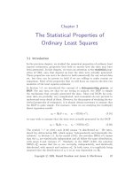
Figure 12.1 Determinants in two dimensions
Consider a simple example in E
2
. Volume in 2 dimensional space is just area.
The simplest area to consider is the unit square, which can be defined as the
parallelogram defined by the two unit basis vectors e
1
and e
2
, where e
i
has
only one nonzero component, in position i. The area of the unit square is, by
definition, 1. The image of the unit square under the mapping defined by a
2 × 2 matrix A is the parallelogram defined by the two columns of the matrix
A[ e
1
e
2
] = AI = A ≡ [ a

1
a
2
],
where a
1
and a
2
are the two columns of A. The area of a parallelogram in
Euclidean geometry is given by base times height, where the length of either
one of the two defining vectors can be taken as the base, and the height is then
the perpendicular distance between the two parallel sides that correspond to
this choice of base. This is illustrated in Figure 12.1.
If we choose a
1
as the base, then, as we can see from the figure, the height is
the length of the vector M
1
a
2
, where M
1
is the orthogonal projection on to
the orthogonal complement of a
1
. Thus the area of the parallelogram defined
by a
1
and a
2

is a
1
M
1
a
2
. By use of Pythagoras’ Theorem and a little
algebra (see Exercise 12.6), it can be seen that
a
1
M
1
a
2
 = |a
11
a
22
− a
12
a
21
|, (12.27)
where a
ij
is the ij
th
element of A. This quantity is the absolute value of
the determinant of A, which we write as |det A|. The determinant itself,
which is defined as a

11
a
22
− a
12
a
21
, can be of either sign. Its signed value
can be written as “det A”, but it is more commonly, and perhaps somewhat
confusingly, written as |A|.
Algebraic expressions for determinants of square matrices of dimension higher
than 2 can be found easily enough, but we will have no need of them. We
will, however, need to make use of some of the properties of determinants.
The principal properties that will matter to us are as follows.
• The determinant of the transpose of a matrix is equal to the determinant
of the matrix itself. That is, |A

| = |A|.
Copyright
c
 1999, Russell Davidson and James G. MacKinnon
504 Multivariate Models
• The determinant of a triangular matrix is the product of its diagonal
elements.
• Since a diagonal matrix can be regarded as a special triangular matrix,
its determinant is also the product of its diagonal elements.
• Since an identity matrix is a diagonal matrix with all diagonal elements
equal to unity, the determinant of an identity matrix is 1.
• If a matrix can be partitioned so as to be block-diagonal, then its deter-
minant is the product of the determinants of the diagonal blocks.

• Interchanging two rows, or two columns, of a matrix leaves the absolute
value of the determinant unchanged but changes its sign.
• The determinant of the product of two square matrices of the same di-
mensions is the product of their determinants, from which it follows that
the determinant of A
−1
is the reciprocal of the determinant of A.
• If a matrix can be inverted, its determinant must be nonzero. Conversely,
if a matrix is singular, its determinant is 0.
• The derivative of log |A| with respect to the ij
th
element a
ij
of A is the
ji
th
element of A
−1
.
Maximum Likelihood Estimation
If we assume that the error terms of an SUR system are normally distributed,
the system can be estimated by maximum likelihood. The model to be esti-
mated can be written as
y
•
= X
•
β
•
+ u

•
, u
•
∼ N(0, Σ ⊗ I
n
). (12.28)
The loglikelihood function for this model is the logarithm of the joint density
of the components of the vector y
•
. In order to derive that density, we must
start with the density of the vector u
•
.
Up to this point, we have not actually written down the density of a random
vector that follows the multivariate normal distribution. We will do so in
a moment. But first, we state a more fundamental result, which extends
the result (10.92) that was proved in Section 10.8 for univariate densities of
transformations of variables to the case of multivariate densities.
Let z be a random m vector with known density f
z
(z), and let x be another
random m vector such that z = h(x), where the deterministic function h(·)
is a one to one mapping of the support of the random vector x, which is a
subset of R
m
, into the support of z . Then the multivariate analog of the result
(10.92) is
f
x
(x) = f

z

h(x)



det J(x)


, (12.29)
where J(x) ≡ ∂h(x)/∂x is the Jacobian matrix of the transformation, that
is, the m × m matrix containing the derivatives of the components of h(x)
with respect to those of x.
Copyright
c
 1999, Russell Davidson and James G. MacKinnon
12.2 Seemingly Unrelated Linear Regressions 505
Using (12.29), it is not difficult to show that, if the m × 1 vector z follows the
multivariate normal distribution with mean vector 0 and covariance matrix Ω,
then its density is equal to
(2π)
−m/2
|Ω|
−1/2
exp

−
1
−
2

z

Ω
−1
z

. (12.30)
Readers are asked to prove a slightly more general result in Exercise 12.8.
For the system (12.28), the function h(·) that gives u
•
as a function of y
•
is
the right-hand side of the equation
u
•
= y
•
− X
•
β
•
. (12.31)
Thus we see that, if there are no lagged dependent variables in the matrix X
•
,
then the Jacobian of the transformation is just the identity matrix, of which
the determinant is 1.
The Jacobian will, in general, be much more complicated if there are lagged
dependent variables, because the elements of X

•
will depend on the elements
of y
•
. However, as readers are invited to check in Exercise 12.10, even though
the Jacobian is, in such a case, not equal to the identity matrix, its determi-
nant is still 1. Therefore, we can ignore the Jacobian when we compute the
density of y
•
. When we substitute (12.31) into (12.30), as the result (12.29)
tells us to do, we find that the density of y
•
is (2π)
−gn/2
times
|Σ ⊗ I
n
|
−1/2
exp

−
1
−
2
(y
•
− X
•
β

•
)

(Σ
−1
⊗ I
n
)(y
•
− X
•
β
•
)

. (12.32)
Jointly maximizing the logarithm of this function with resp ect to β
•
and the
elements of Σ gives the ML estimator of the SUR system.
The argument of the exponential function in (12.32) plays the same role for a
multivariate linear regression model as the sum of squares term plays in the
loglikelihood function (10.10) for a linear regression model with IID normal
errors. In fact, it is clear from (12.32) that maximizing the loglikelihood with
respect to β
•
for a given Σ is equivalent to minimizing the function
(y
•
− X

•
β
•
)

(Σ
−1
⊗ I
n
)(y
•
− X
•
β
•
)
with respect to β
•
. This expression is just the criterion function (12.11) that
is minimized in order to obtain the GLS estimator (12.09). Therefore, the
ML estimator
ˆ
β
ML
•
must have exactly the same form as (12.09), with the
matrix Σ replaced by its ML estimator
ˆ
Σ
ML

, which we will derive shortly.
It follows from (12.32) that the loglikelihood function (Σ, β
•
) for the model
(12.28) can be written as
−
gn
−−
2
log 2π −
1
−
2
log |Σ ⊗ I
n
| −
1
−
2
(y
•
− X
•
β
•
)

(Σ
−1
⊗ I

n
)(y
•
− X
•
β
•
).
Copyright
c
 1999, Russell Davidson and James G. MacKinnon
506 Multivariate Models
The properties of determinants set out in the previous subsection can be used
to show that the determinant of Σ ⊗I
n
is |Σ|
n
; see Exercise 12.11. Thus this
loglikelihood function simplifies to
−
gn
−−
2
log 2π −
n
−
2
log |Σ| −
1
−

2
(y
•
− X
•
β
•
)

(Σ
−1
⊗ I
n
)(y
•
− X
•
β
•
). (12.33)
We have already seen how to maximize the function (12.33) with respect to β
•
conditional on Σ. Now we want to maximize it with respect to Σ.
Maximizing (Σ, β
•
) with respect to Σ is of course equivalent to maximizing it
with respect to Σ
−1
, and it turns out to be technically simpler to differentiate
with respect to the elements of the latter matrix. Note first that, since the

determinant of the inverse of a matrix is the reciprocal of the determinant
of the matrix itself, we have − log |Σ| = log |Σ
−1
|, so that we can readily
express all of (12.33) in terms of Σ
−1
rather than Σ.
It is obvious that the derivative of any p × q matrix A with respect to its ij
th
element is the p × q matrix E
ij
, all the elements of which are 0, except for
the ij
th
, which is 1. Recall that we write the ij
th
element of Σ
−1
as σ
ij
. We
therefore find that
∂Σ
−1
∂σ
ij
= E
ij
, (12.34)
where in this case E

ij
is a g ×g matrix. We remarked in our earlier discussion
of determinants that the derivative of log |A| with respect to a
ij
is the ji
th
element of A
−1
. Armed with this result and (12.34), we see that the derivative
of the loglikelihood function (Σ, β
•
) with respect to the element σ
ij
is
∂(Σ, β
•
)
∂σ
ij
=
n
−
2
σ
ij
−
1
−
2
(y

•
− X
•
β
•
)

(E
ij
⊗ I
n
)(y
•
− X
•
β
•
). (12.35)
The Kronecker product E
ij
⊗ I
n
has only one nonzero block containing I
n
. It
is easy to conclude from this that
(y
•
− X
•

β
•
)

(E
ij
⊗ I
n
)(y
•
− X
•
β
•
) = (y
i
− X
i
β
i
)

(y
j
− X
j
β
j
).
By equating the partial derivative (12.35) to zero, we find that the ML esti-

mator ˆσ
ML
ij
is
ˆσ
ML
ij
=
1
−
n
(y
i
− X
i
ˆ
β
ML
i
)

(y
j
− X
j
ˆ
β
ML
j
).

If we define the n × g matrix U(β
•
) to have i
th
column y
i
− X
i
β
i
, then we
can conveniently write the ML estimator of Σ as follows:
ˆ
Σ
ML
=
1
−
n
U

(
ˆ
β
ML
•
)U (
ˆ
β
ML

•
). (12.36)
This lo oks like equation (12.17), which defines the covariance matrix used in
feasible GLS estimation. Equations (12.36) and (12.17) have exactly the same
Copyright
c
 1999, Russell Davidson and James G. MacKinnon
12.2 Seemingly Unrelated Linear Regressions 507
form, but they are based on different matrices of residuals. Equation (12.36)
and equation (12.09) evaluated at
ˆ
Σ
ML
, that is
ˆ
β
ML
•
=

X
•

(
ˆ
Σ
−1
ML
⊗ I
n

)X
•

−1
X
•

(
ˆ
Σ
−1
ML
⊗ I
n
)y
•
, (12.37)
together define the ML estimator for the model (12.28).
Equations (12.36) and (12.37) are exactly the ones that are used by the con-
tinuously updated GMM estimator to update the estimates of Σ and β
•
,
respectively. It follows that, if the continuous updating procedure converges,
it converges to the ML estimator. Consequently, we can estimate the covar-
iance matrix of
ˆ
β
ML
•
in the same way as for the GLS or GMM estimator, by

the formula

Var(
ˆ
β
ML
•
) =

X
•

(
ˆ
Σ
−1
ML
⊗ I
n
)X
•

−1
. (12.38)
It is also possible to estimate the covariance matrix of the estimated con-
temporaneous covariance matrix,
ˆ
Σ
ML
, although this is rarely done. If the

elements of Σ are stacked in a vector of length g
2
, a suitable estimator is

Var

Σ(
ˆ
β
ML
•
)

=
2
−
n
Σ(
ˆ
β
ML
•
) ⊗ Σ(
ˆ
β
ML
•
). (12.39)
Notice that the estimated variance of any diagonal element of Σ is just twice
the square of that element, divided by n. This is precisely what is obtained

for the univariate case in Exercise 10.10. As with that result, the asymptotic
validity of (12.39) depends critically on the assumption that the error terms
are multivariate normal.
As we saw in Chapter 10, ML estimators are consistent and asymptotically
efficient if the underlying model is correctly sp ecified. It may therefore seem
that the asymptotic efficiency of the ML estimator (12.37) depends critically
on the multivariate normality assumption. However, the fact that the ML esti-
mator is identical to the continuously updated efficient GMM estimator means
that it is in fact efficient in the same sense as the latter. When the errors are
not normal, the estimator is more properly termed a QMLE (see Section 10.4).
As such, it is consistent, but not necessarily efficient, under assumptions about
the error terms that are no stronger than those needed for feasible GLS to be
consistent. Moreover, if the stronger assumptions made in (12.02) hold, even
without normality, then the estimator (12.38) of Var (
ˆ
β
ML
•
) is asymptotically
valid. If the error terms are not normal, it would be necessary to have infor-
mation about their actual distribution in order to derive an estimator with a
smaller asymptotic variance than (12.37).
It is of considerable theoretical interest to concentrate the loglikelihood func-
tion (12.33) with respect to Σ. In order to do so, we use the first-order condi-
tions that led to (12.36) to define Σ(β
•
) as the matrix that maximizes (12.33)
for given β
•
. We find that

Σ(β
•
) ≡
1
−
n
U

(β
•
)U (β
•
).
Copyright
c
 1999, Russell Davidson and James G. MacKinnon
508 Multivariate Models
A calculation of a type that should now be familiar then shows that
(y
•
− X
•
β
•
)

(Σ
−1
⊗ I
n

)(y
•
− X
•
β
•
)
=
g

i=1
g

j=1
σ
ij
(y
i
− X
i
β
i
)

(y
j
− X
j
β
j

).
(12.40)
When σ
ij
= σ
ij
(β
•
), which denotes the ij
th
element of Σ
−1
(β
•
), the right-
hand side of equation (12.40) is
g

i=1
g

j=1
σ
ij
(β
•
)

U


(β
•
)U (β
•
)

ij
= n
g

i=1
g

j=1
σ
ij
(β
•
)σ
ij
(β
•
)
= n
g

i=1
(I
g
)

ii
= n Tr(I
g
) = gn,
where we have made use of the trace operator, which sums the diagonal ele-
ments of a square matrix; see Section 2.6. By substituting this result into
expression (12.33), we see that the concentrated loglikelihood function can be
written as
−
gn
−−
2
(log 2π + 1) −
n
−
2
log



1
−
n
U

(β
•
)U (β
•
)




. (12.41)
This expression depends on the data only through the determinant of the
covariance matrix of the residuals. It is the multivariate generalization of the
concentrated loglikelihood function (10.11) that we obtained in Section 10.2
in the univariate case. We saw there that the concentrated function depends
on the data only through the sum of squared residuals.
It is quite possible to minimize the determinant in (12.41) with respect to β
•
directly. It may or may not be numerically simpler to do so than to solve the
coupled equations (12.37) and (12.36).
We saw in Section 3.6 that the squared residuals of a univariate regression
model tend to be smaller than the squared error terms, because least squares
estimates make the sum of squared residuals as small as possible. For a similar
reason, the residuals from ML estimation of a multivariate regression model
tend to be too small and too highly correlated with each other. We observe
both effects, because the determinant of Σ can be made smaller either by
reducing the sums of squared residuals associated with the individual equa-
tions or by increasing the correlations among the residuals. This is likely to
be most noticeable when g and/or the k
i
are large relative to n.
Although feasible GLS and ML with the assumption of normally distributed
errors are by far the most commonly used methods of estimating linear SUR
systems, they are by no means the only ones that have been proposed. For
fuller treatments, a classic reference on linear SUR systems is Srivastava and
Giles (1987), and a useful recent survey paper is Fiebig (2001).
Copyright

c
 1999, Russell Davidson and James G. MacKinnon
12.3 Systems of Nonlinear Regressions 509
12.3 Systems of Nonlinear Regressions
Many multivariate regression models are nonlinear. For example, economists
routinely estimate demand systems, in which the shares of consumer expen-
diture on various classes of goods and services are explained by incomes,
prices, and perhaps other explanatory variables. Demand systems may be
estimated using aggregate time-series data, cross-section data, or mixed time-
series/cross-section (panel) data on households.
1
The multivariate nonlinear regression model is a system of nonlinear regres-
sions which can be written as
y
ti
= x
ti
(β) + u
ti
, t = 1, . . . , n, i = 1, . . . , g. (12.42)
Here y
ti
is the t
th
observation on the i
th
dependent variable, x
ti
(β) is the t
th

observation on the regression function which determines the conditional mean
of that dependent variable, β is a k vector of parameters to be estimated,
and u
ti
is an error term which is assumed to have mean zero conditional
on all the explanatory variables that implicitly appear in all the regression
functions x
tj
(β), j = 1, . . . , g. In the demand system case, y
ti
would be the
share of expenditure on commodity i for observation t, and the explanatory
variables would include prices and income. We assume that the error terms
in (12.42), like those in (12.01), satisfy assumption (12.02). They are serially
uncorrelated, homoskedastic within each equation, and have contemporaneous
covariance matrix Σ with typical element σ
ij
.
The equations of the system (12.42) can also be written using essentially
the same notation as we used for univariate nonlinear regression models in
Chapter 6. If, for each i = 1, . . . , g, the n vectors y
i
, x
i
(β), and u
i
are
defined to have typical elements y
ti
, u

ti
, and x
ti
(β), respectively, then the
entire system can be expressed as
y
i
= x
i
(β) + u
i
, E(u
i
u
j

) = σ
ij
I
n
, i, j = 1, . . . , g. (12.43)
We have written (12.42) and (12.43) in such a way that there is just a single
vector of parameters, denoted β. Every individual parameter may, at least in
principle, appear in every equation, although that is rare in practice. In the
demand systems case, however, some but not all of the parameters typically do
appear in every equation of the system. Thus systems of nonlinear regressions
very often involve cross-equation restrictions.
Multivariate nonlinear regression models can be estimated in essentially the
same way as the multivariate linear regression mo del (12.01). Feasible GLS
1

The literature on demand systems is vast; see, among many others, Christensen,
Jorgenson, and Lau (1975), Barten (1977), Deaton and Muellbauer (1980),
Pollak and Wales (1981, 1987), Browning and Meghir (1991), Lewbel (1991),
and Blundell, Browning, and Meghir (1994).
Copyright
c
 1999, Russell Davidson and James G. MacKinnon
510 Multivariate Models
and maximum likelihood are both commonly used. The results we obtained
in the previous section still apply, provided they are modified to allow for the
nonlinearity of the regression functions and for cross-equation restrictions.
Our discussion will therefore be quite brief.
Estimation
We saw in Section 7.3 that nonlinear GLS estimates can be obtained either by
minimizing the criterion function (7.13) or, equivalently, by solving the set of
first-order conditions (7.14). For the multivariate nonlinear regression model
(12.42), the criterion function can be written so that it looks very much like
expression (12.11). Let y
•
once again denote a gn vector of the y
i
stacked
vertically, and let x
•
(β) denote a gn vector of the x
i
(β) stacked in the same
way. The criterion function (7.13) then becomes

y

•
− x
•
(β)


(Σ
−1
⊗ I
n
)

y
•
− x
•
(β)

. (12.44)
Minimizing (12.44) with respect to β yields nonlinear GLS estimates which,
by the results of Section 7.2, are consistent and asymptotically efficient under
standard regularity conditions.
The first-order conditions for the minimization of (12.44) give rise to the
following moment conditions, which have a very similar form to the moment
conditions (12.12) that we found for the linear case:
X
•

(β)(Σ
−1

⊗ I
n
)

y
•
− x
•
(β)

= 0. (12.45)
Here, the gn× k matrix X
•
(β) is a matrix of partial derivatives of the x
ti
(β).
If the n × k matrices X
i
(β) are defined, just as in the univariate case, so
that the tj
th
element of X
i
(β) is ∂x
ti
(β)/∂β
j
, for t = 1, . . . , n, j = 1, . . . , k,
then X
•

(β) is the matrix formed by stacking the X
i
(β) vertically. Except in
the special case in which each parameter appears in only one equation of the
system, X
•
(β) does not have the block-diagonal structure of X
•
in (12.05).
Despite this fact, it is not hard to show that the moment conditions (12.45)
can be expressed in a compact form like (12.16), but with a double sum. As
readers are asked to check in Exercise 12.12, we obtain estimating equations
of the form
g

i=1
g

j=1
σ
ij
X
i

(β)

y
j
− x
j

(β)

= 0. (12.46)
The vector
ˆ
β
GLS
that solves these equations is the nonlinear GLS estimator.
Adapting expression (7.05) to the model (12.43) gives the standard estimate
of the covariance matrix of the nonlinear GLS estimator, namely,

Var(
ˆ
β
GLS
) =

X
•

(
ˆ
β
GLS
)(Σ
−1
⊗ I
n
)X
•

(
ˆ
β
GLS
)

−1
. (12.47)
Copyright
c
 1999, Russell Davidson and James G. MacKinnon
12.3 Systems of Nonlinear Regressions 511
This can also be written (see Exercise 12.12 again) as

Var(
ˆ
β
GLS
) =

g

i=1
g

j=1
σ
ij
X
i


(
ˆ
β
GLS
)X
j
(
ˆ
β
GLS
)

−1
. (12.48)
Feasible GLS estimation works in essentially the same way for nonlinear mul-
tivariate regression models as it does for linear ones. The individual equations
of the system are first estimated separately by either ordinary or nonlinear
least squares, as appropriate. The residuals are then grouped into an n × g
matrix
ˆ
U, and equation (12.17) is used to obtain the estimate
ˆ
Σ. We can
then replace Σ by
ˆ
Σ in the GLS criterion function (12.44) or in the moment
conditions (12.45) to obtain the feasible GLS estimator
ˆ
β

F
. We may also
use a continuously updated estimator, alternately updating our estimates of
β and Σ. If this iterated feasible GLS procedure converges, we will have
obtained ML estimates, although there may well be more computationally
attractive ways to do so.
Maximum likelihood estimation under the assumption of normality is very
popular for multivariate nonlinear regression models. For the system (12.42),
the loglikelihood function can be written as
−
gn
−−
2
log 2π −
n
−
2
log |Σ| −
1
−
2

y
•
− x
•
(β)


(Σ

−1
⊗ I
n
)

y
•
− x
•
(β)

. (12.49)
This is the analog of the loglikelihood function (12.33) for the linear case.
Maximizing (12.49) with respect to β for given Σ is equivalent to minimizing
the criterion function (12.44) with respect to β, and so the first-order condi-
tions are equations (12.45). Maximizing (12.49) with respect to
Σ
for given
β
leads to first-order conditions that can be written as
Σ(β) =
1
−
n
U

(β)U(β),
in exactly the same way as the maximization of (12.33) with respect to Σ
led to equation (12.36). Here the n × g matrix U (β) is defined so that its
i

th
column is y
i
− x
i
(β).
Thus the estimating equations that define the ML estimator are
X
•

(
ˆ
β
ML
)(
ˆ
Σ
−1
ML
⊗ I
n
)

y
•
− x
•
(
ˆ
β

ML
)

= 0, and
ˆ
Σ
ML
=
1
−
n
U

(
ˆ
β
ML
)U (
ˆ
β
ML
).
(12.50)
As in the linear case, these are also the estimating equations for the continu-
ously updated GMM estimator. The covariance matrix of
ˆ
β
ML
is, of course,
given by either of the formulas (12.47) or (12.48) evaluated at

ˆ
β
ML
and
ˆ
Σ
ML
.
The loglikelihood function concentrated with respect to Σ can b e written,
Copyright
c
 1999, Russell Davidson and James G. MacKinnon
512 Multivariate Models
just like expression (12.41), as
−
gn
−−
2
(log 2π + 1) −
n
−
2
log



1
−
n
U


(β)U(β)



. (12.51)
As in the linear case, it may or may not be numerically easier to maximize the
concentrated function directly than to solve the estimating equations (12.50).
The Gauss-Newton Regression
The Gauss-Newton regression can be very useful in the context of multivariate
regression models, both linear and nonlinear. The starting point for setting
up the GNR for both types of multivariate model is equation (7.15), the GNR
for the standard univariate model y = x(β) + u, with Var(u) = Ω. This
GNR takes the form
Ψ


y − x(β)

= Ψ

X(β)b + residuals,
where, as usual, X(β) is the matrix of partial derivatives of the regression
functions, and Ψ is such that Ψ Ψ

= Ω
−1
.
Expressed as a univariate regression, the multivariate model (12.43) becomes
y

•
= x
•
(β) + u
•
, Var(u
•
) = Σ ⊗ I
n
. (12.52)
If we now define the g × g matrix Ψ such that Ψ Ψ

= Σ
−1
, it is clear that
(Ψ ⊗ I
n
)(Ψ ⊗ I
n
)

= (Ψ ⊗ I
n
)(Ψ

⊗ I
n
) = (Ψ Ψ

⊗ I

n
) = Σ
−1
⊗ I
n
,
where the last expression is the inverse of the covariance matrix of u
•
.
From (7.15), the GNR corresponding to (12.52) is therefore
(Ψ

⊗ I
n
)

y
•
− x
•
(β)

= (Ψ

⊗ I
n
)X
•
(β)b + residuals. (12.53)
The gn × k matrix X

•
(β) is the matrix of partial derivatives that we already
defined for use in the moment conditions (12.45). Observe that, as required
for a properly defined artificial regression, the inner product of the regressand
with the matrix of regressors yields the left-hand side of the moment condi-
tions (12.45), and the inverse of the inner product of the regressor matrix with
itself has the same form as the covariance matrix (12.47).
The Gauss-Newton regression (12.53) can be useful in a number of contexts.
It provides a convenient way to solve the estimating equations (12.45) in
order to obtain an estimate of β for given Σ, and it automatically computes
the covariance matrix estimate (12.47) as well. Because feasible GLS and
ML estimation are algebraically identical as regards the estimation of the
parameter vector β, the GNR is useful in both contexts. In practice, it is
frequently used to calculate test statistics for restrictions on
β
; see Section 6.7.
Another important use is to impose cross-equation restrictions after equation-
by-equation estimation. For this purpose, the multivariate GNR is just as
useful for linear systems as for nonlinear ones; see Exercise 12.13.
Copyright
c
 1999, Russell Davidson and James G. MacKinnon
12.4 Linear Simultaneous Equations Models 513
12.4 Linear Simultaneous Equations Models
In Chapter 8, we dealt with instrumental variables estimation of a single
equation in which some of the explanatory variables are endogenous. As we
noted there, it is necessary to have information about the data-generating
process for all of the endogenous variables in order to determine the optimal
instruments. However, we actually dealt with only one equation, or at least
only one equation at a time. The model that we consider in this section and

the next, namely, the linear simultaneous equations model, extends what we
did in Chapter 8 to a model in which all of the endogenous variables have the
same status. Our objective is to obtain efficient estimates of the full set of
parameters that appear in all of the simultaneous equations.
The Model
The i
th
equation of a linear simultaneous system can be written as
y
i
= X
i
β
i
+ u
i
= Z
i
β
1i
+ Y
i
β
2i
+ u
i
, (12.54)
where X
i
is an n × k

i
matrix of explanatory variables that can be partitioned
as X
i
= [ Z
i
Y
i
]. Here Z
i
is an n × k
1i
matrix of variables that are assumed
to be exogenous or predetermined, and Y
i
is an n × k
2i
matrix of endogenous
variables, with k
1i
+ k
2i
= k
i
. The k
i
vector β
i
of parameters can be parti-
tioned as [β

1i
.
.
.
.
β
2i
] to conform with the partitioning of X. The g endogenous
variables y
1
through y
g
are assumed to be jointly generated by g equations of
the form (12.54). The number of exogenous or predetermined variables that
appear anywhere in the system is l. This implies that k
1i
≤ l for all i.
2
We make the standard assumption (12.02) about the error terms. Thus we
allow for contemporaneous correlation, but not for heteroskedasticity or serial
correlation. It is, of course, quite possible to allow for these extra complica-
tions, but they are are not admitted in the context of the model currently
under discussion, which thus has a distinctly classical flavor, as befits a model
that has inspired a long and distinguished literature.
Except for the explicit distinction between endogenous and predetermined ex-
planatory variables, equation (12.54) looks very much like the typical equation
(12.01) of an SUR system. However, there is one important difference, which
is concealed by the notation. It is that, as with the simple demand-supply
model of Section 8.2, the dependent variables y
i

are not necessarily distinct.
2
Readers should be warned that the notation we have introduced in equation
(12.54) is not universal. In particular, some authors reverse the definitions of
X
i
and Z
i
and then define X to be the n × l matrix of all the exogenous
and predetermined variables, which we will denote below by W. Our notation
emphasizes the similarities between the linear simultaneous equations model
(12.54) and the linear SUR system (12.01), as well as making it clear that W
plays the role of a matrix of instruments.
Copyright
c
 1999, Russell Davidson and James G. MacKinnon
514 Multivariate Models
Since equations (12.54) form a simultaneous system, it is arbitrary which one
of the endogenous variables is put on the left-hand side with a coefficient of 1,
at least in any equation in which more than one endogenous variable appears.
It is a matter of simple algebra to select one of the variables in the matrix Y
i
,
take it over to the left-hand side while taking y
i
over to the right, and then
rescale the coefficients so that the selected variable has a coefficient of 1. This
point can be important in practice.
Just as we did with the linear SUR model, we can convert the system of
equations (12.54) to a single equation by stacking them vertically. As before,

the gn vectors y
•
and u
•
consist of the y
i
and the u
i
, respectively, stacked
vertically. The gn × k matrix X
•
, where k = k
1
+ . . . + k
g
, is defined to be
a block-diagonal matrix with diagonal blocks X
i
, just as in equation (12.05).
The full system can then be written as
y
•
= X
•
β
•
+ u
•
, E(u
•

u
•

) = Σ ⊗ I
n
, (12.55)
where the k vector β
•
is formed by stacking the β
i
vertically. As before, the
g × g matrix Σ is the contemporaneous covariance matrix of the error terms.
The true value of β
•
will be denoted β
0
•
.
Efficient GMM Estimation
One of the main reasons for estimating a full system of equations is to obtain
an efficiency gain relative to single-equation estimation. In Section 9.2, we
saw how to obtain the most efficient possible estimator for a single equation in
the context of efficient GMM estimation. The theoretical moment conditions
that lead to such an estimator are given in equation (9.18), which we rewrite
here for easy reference:
E

¯
X


Ω
−1
(y − Xβ)

= 0. (9.18)
Because we are assuming that there is no serial correlation, these moment
conditions are also valid for the linear simultaneous equations model (12.54).
We simply need to reinterpret them in terms of that model.
In reinterpreting the moment conditions (9.18), it is clear that y
•
will replace
the vector y, X
•
β
•
will replace the vector Xβ, and Σ
−1
⊗ I
n
will replace the
matrix Ω
−1
. What is not quite so clear is what will replace
¯
X. Recall that
¯
X
in (9.18) is the matrix defined row by row so as to contain the expectations of
the explanatory variables for each observation conditional on the information
that is predetermined for that observation. We need to obtain the matrix that

corresponds to
¯
X in equation (9.18) for the model (12.55).
Let W denote an n × l matrix of exogenous and predetermined variables, the
columns of which are all of the linearly independent columns of the Z
i
. For
these variables, the expectations conditional on predetermined information
are just the variables themselves. Thus we only need worry about the endo-
genous explanatory variables. Because their joint DGP is given by the system
Copyright
c
 1999, Russell Davidson and James G. MacKinnon
12.4 Linear Simultaneous Equations Models 515
of linear equations (12.54), it must be possible to solve these equations for
the endogenous variables as functions of the predetermined variables and the
error terms. Since these equations are linear and have the same form for all
observations, the solution must have the form
y
i
= Wπ
i
+ error terms, (12.56)
where π
i
is an l vector of parameters that are, in general, nonlinear functions
of the parameters β
•
. As the notation indicates, the variables contained in
the matrix W serve as instrumental variables for the estimation of the model

parameters. Later, we will investigate more fully the nature of the π
i
. We
pay little attention to the error terms, because our objective is to compute
the conditional expectations of the elements of the y
i
, and we know that each
of the error terms must have expectation 0 conditional on all the exogenous
and predetermined variables.
The vector of conditional expectations of the elements of y
i
is just Wπ
i
. Since
equations (12.56) take the form of linear regressions with exogenous and pre-
determined explanatory variables, OLS estimates of the π
i
are consistent. As
we saw in Section 12.2, they are also efficient, even though the error terms
will generally display contemporaneous correlation, because the same regres-
sors appear in every equation. Thus we can replace the unknown π
i
by their
OLS estimates based on equations (12.56). This means that the conditional
expectations of the vectors y
i
are estimated by the OLS fitted values, that
is, the vectors W
ˆ
π

i
= P
W
y
i
. When this is done, the matrices that contain
the estimates of the conditional expectations of the elements of the X
i
can be
written as
ˆ
X
i
≡ [ Z
i
P
W
Y
i
] = P
W
[ Z
i
Y
i
] = P
W
X
i
. (12.57)

We write
ˆ
X
i
rather than
¯
X
i
because the unknown conditional expectations
are estimated. The step from the second to the third expression in (12.57) is
possible because all the columns of all the Z
i
are, by construction, contained
in the span of the columns of W.
We are now ready to construct the matrix to be used in place of
¯
X in (9.18).
It is the block-diagonal gn × k matrix
ˆ
X
•
, with diagonal blocks the
ˆ
X
i
. This
allows us to write the estimating equations for efficient GMM estimation as
ˆ
X
•


(Σ
−1
⊗ I
n
)(y
•
− X
•
β
•
) = 0. (12.58)
These equations, which are the empirical versions of the theoretical moment
conditions (9.18), can be rewritten in several other ways. In particular, they
can be written in the form



σ
11
X
1

P
W
· · · σ
1g
X
1


P
W
.
.
.
.
.
.
.
.
.
σ
g1
X
g

P
W
· · · σ
gg
X
g

P
W







y
1
− X
1
β
1
.
.
.
y
g
− X
g
β
g



= 0,
Copyright
c
 1999, Russell Davidson and James G. MacKinnon
516 Multivariate Models
by analogy with equation (12.13), and in the form
g

j=1
σ
ij

X
i

P
W
(y
j
− X
j
β
j
) = 0, i = 1, . . . , g, (12.59)
by analogy with equation (12.16). It is also straightforward to check (see
Exercise 12.14) that they can be written as
X
•

(Σ
−1
⊗ P
W
)(y
•
− X
•
β
•
) = 0, (12.60)
from which it follows immediately that equations (12.58) are equivalent to the
first-order conditions for the minimization of the criterion function

(y
•
− X
•
β
•
)

(Σ
−1
⊗ P
W
)(y
•
− X
•
β
•
). (12.61)
The efficient GMM estimator
ˆ
β
GMM
•
defined by (12.60) is the analog for a
linear simultaneous equations system of the GLS estimator (12.09) for an
SUR system.
The asymptotic covariance matrix of
ˆ
β

GMM
•
can readily be obtained from
expression (9.29). In the notation of (12.58), we find that
Var

plim
n→∞
n
1/2
(
ˆ
β
GMM
•
− β
0
•
)

= plim
n→∞

1
−
n
ˆ
X
•


(Σ
−1
⊗ I
n
)
ˆ
X
•

−1
. (12.62)
This covariance matrix can also be written, in the notation of (12.60), as
plim
n→∞

1
−
n
X
•

(Σ
−1
⊗ P
W
)X
•

−
1

. (12.63)
Of course, the estimator
ˆ
β
GMM
•
is not feasible if, as is almost always the case,
the matrix Σ is unknown. However, it is obvious that we can deal with this
problem by using a procedure analogous to feasible GLS estimation of an SUR
system. We will return to this issue at the end of this section.
Two Special Cases
If the matrix Σ is diagonal, then equations (12.59) simplify to
σ
ii
X
i

P
W
(y
i
− X
i
β
i
) = 0, i = 1, . . . , g. (12.64)
The factors of σ
ii
have no influence on the solutions to these equations, which
are therefore just the generalized IV, or 2SLS, estimators for each of the

equations of the system treated individually, with a common matrix W of
instrumental variables. This result is the analog of what we found for an SUR
system with diagonal Σ. Here it is the equation-by-equation IV estimator
that takes the place of the equation-by-equation OLS estimator.
Copyright
c
 1999, Russell Davidson and James G. MacKinnon