Class Notes in Statistics and Econometrics Part 6 pot

Bạn đang xem bản rút gọn của tài liệu. Xem và tải ngay bản đầy đủ của tài liệu tại đây (499.23 KB, 45 trang )

CHAPTER 11
The Regression Fallacy
Only for the sake of this exercise we will assume that “intelligence” is an innate
prop e rty of individuals and can be represented by a real number z. If one picks at
random a student entering the U of U, the intelligence of this student is a random
variable which we assume to be normally distributed with mean µ and standard
deviation σ. Also assume every student has to take two intelligence tests, the ﬁrst
at the beginning of his or her studies, the other half a year later. The outcomes of
these tests are x and y. x and y measure the intelligence z (which is assumed to be
the same in both tests) plus a random error ε and δ, i.e.,
x = z + ε(11.0.14)
y = z + δ(11.0.15)
309
310 11. THE REGRESSION FALLACY
Here z ∼ N (µ, τ
2
), ε ∼ N(0, σ
2
), and δ ∼ N (0, σ
2
) (i.e., we assume that both errors
have the same variance). The three variables ε, δ, and z are independent of each
other. Therefore x and y are jointly normal. var[x] = τ
2
+ σ
2
, var[y] = τ
2
+ σ
2
,

cov[x, y] = cov[z + ε, z +δ] = τ
2
+ 0 + 0 + 0 = τ
2
. Therefore ρ =
τ
2
τ
2
+σ
2
. The contour
lines of the joint density are ellipses with center (µ, µ) whose main axes are the lines
y = x and y = −x in the x, y-plane.
Now what is the conditional mean? Since var[x] = var[y], (10.3.17) gives the
line E[y|x=x] = µ + ρ(x − µ), i.e., it is a line which goes through the center of the
ellipses but which is ﬂatter than the line x = y representing the real underlying linear
relationship if there are no errors. Geometrically one can get it as the line which
intersects each ellipse exactly where the ellipse is vertical.
Therefore, the parameters of the best prediction of y on the basis of x are not
the parameters of the underlying relationship. Why not? Because not only y but
also x is subject to errors. As sume you pick an individual by random, and it turns
out that his or her ﬁrst test result is very much higher than the average. Then it is
more likely that this is an individual which was lucky in the ﬁrst exam, and his or
her true IQ is lower than the one measured, than that the individual is an Einstein
who had a bad day. This is simply because z is normally distributed, i.e., among the
students entering a given University, there are more individuals with lower IQ’s than
Einsteins. In order to make a good prediction of the result of the second test one
11. THE REGRESSION FALLACY 311
must make allowance for the fact that the individual’s IQ is most likely lower than

his ﬁrst score indicated, therefore one will predict the second score to be lower than
the ﬁrst score. The converse is true for individuals who scored lower than average,
i.e., in your prediction you will do as if a “regression towards the mean” had taken
place.
The next important point to note here is: the “true regression line,” i.e., the
prediction line, is uniquely determined by the joint distribution of x and y. However
the line representing the underlying relationship can only be determined if one has
information in addition to the joint density, i.e., in addition to the observations.
E.g., assume the two tests have diﬀerent standard deviations, which may be the case
simply because the second test has more questions and is therefore more accurate.
Then the underlying 45
◦
line is no longer one of the main axes of the ellipse! To be
more precise, the underlying line can only be identiﬁed if one knows the ratio of the
variances, or if one knows one of the two variances. Without any knowledge of the
variances, the only thing one can say about the underlying line is that it lies between
the line predicting y on the basis of x and the line predicting x on the basis of y.
The name “regression” stems from a confusion between the prediction line and
the real underlying relationship. Francis Galton, the cousin of the famous Darwin,
measured the height of fathers and sons, and concluded from his e vidence that the
heights of sons tended to be closer to the average height than the height of the
312 11. THE REGRESSION FALLACY
fathers, a purported law of “regression towards the mean.” Problem 180 illustrates
this:
Problem 180. The evaluation of two intelligence tests, one at the beginning
of the semester, one at the end, gives the following disturbing outcome: While the
underlying intelligence during the ﬁrst test was z ∼ N(100, 20), it changed between
the ﬁrst and second test due to the learning experience at the university. If w is the
intelligence of each student at the second test, it is connected to his intelligence z
at the ﬁrst test by the formula w = 0.5z + 50, i.e., those students with intelligence

below 100 gained, but those students with intelligence above 100 lost. (The errors
of both intelligence tests are normally distributed with expected value zero, and the
variance of the ﬁrst intelligence test was 5, and that of the second test, which had
more questions, was 4. As usual, the errors are independent of each other and of the
actual intelligence.)
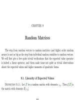
• a. 3 points If x and y are the outcomes of the ﬁrst and second intelligence
test, compute E[x], E[y], var[x], var[y], and the correlation coeﬃcient ρ = corr[x, y].
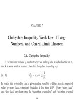
Figure 1 shows an equi-density line of their joint distribution; 95% of the probability
mass of the test results are inside this ellipse. Draw the line w = 0.5z + 50 into
Figure 1.
Answer. We know z ∼ N(100, 20); w = 0.5z + 50; x = z + ε; ε ∼ N(0, 4); y = w + δ;
δ ∼ N(0, 5); therefore E[x] = 100; E[y] = 100; var[x] = 20 + 5 = 25; var[y] = 5 + 4 = 9;
11. THE REGRESSION FALLACY 313
cov[x, y] = 10; corr[x, y] = 10/15 = 2/3. In matrix notation
(11.0.16)

x
y

∼ N


100
100

,

25 10
10 9



The line y = 50 + 0.5x goes through the points (80, 90) and (120, 110). 
• b. 4 points Compute E[y|x=x] and E[x|y=y]. The ﬁrst is a linear function of
x and the second a linear function of y. Draw the two lines representing these linear
functions into Figure 1. Use (10.3.18) for this.
Answer.
E[y|x=x] = 100 +
10
25
(x − 100) = 60 +
2
5
x(11.0.17)
E[x|y=y] = 100 +
10
9
(y − 100) = −
100
9
+
10
9
y.(11.0.18)
The line y = E[y|x=x] goes th roug h the points (80, 92) and (120, 108) at the edge of Figure 1; it
intersects the ellipse where it is vertical. The line x = E[x|y=y] goes through the points (80, 82) and
(120, 118), which are the corner points of Figure 1; it intersects the ellipse where it is horizontal.
The two lines intersect in the center of the ellipse, i.e., at the p oint (100, 100).

• c. 2 points Another researcher says that w =
6

10
z + 40, z ∼ N(100,
100
6
),
ε ∼ N (0,
50
6
), δ ∼ N(0, 3). Is this compatible with the data?
314 11. THE REGRESSION FALLACY
Answer. Yes, it is compatible: E[x] = E[z]+E[ε] = 100; E[y] = E[w]+E[δ] =
6
10
100+40 = 100;
var[x] =
100
6
+
50
6
= 25; var[y] =

6
10

2
var[z] + var[δ] =
63
100
100

6
+ 3 = 9; cov[x, y] =
6
10
var[z] =
10. 
• d. 4 points A third researcher asserts that the IQ of the students really did not
change. He says w = z, z ∼ N(100, 5), ε ∼ N (0, 20), δ ∼ N(0, 4). Is this compatible
with the data? Is there unambiguous evidence in the data that the IQ declined?
Answer. This is not compatible. This scenario gets everything right except the covariance:
E[x] = E[z] + E[ε] = 100; E[y] = E[z] + E[δ] = 100; var[x] = 5 + 20 = 25; var[y] = 5 + 4 = 9;
cov[x, y] = 5. A scenario in which both tests have same underlying intelligence cannot be found.
Since the two conditional expectations are on the same side of the diagonal, the hypothesis that
the intelligence did not change between the two tests is not consistent with the joint distribution
of x and y. The diagonal goes through the points (82, 82) and (118, 118), i.e., it intersects the two
horizontal boundaries of Figure 1. 
We just showed that the parameters of the true underlying relationship cannot
be inferred from the data alone if there are errors in both variables. We also showed
that this lack of identiﬁcation is not complete, because one can specify an interval
which in the plim contains the true parameter value.
Chapter 53 has a much more detailed discussion of all this. There we will see
that this lack of identiﬁcation can be removed if more information is available, i.e., if
one knows that the two e rror variances are equal, or if one knows that the regress ion
11. THE REGRESSION FALLACY 315
has zero intercept, etc. Question 181 shows that in this latter case, the OLS estimate
is not consistent, but other estimates exist that are consistent.
Problem 181. [Fri57, chapter 3] According to Friedman’s permanent income
hypothesis, drawing at random families in a given country and asking them about
their income y and consumption c can be modeled as the independent observations of
two random variables which satisfy

y = y
p
+ y
t
,(11.0.19)
c = c
p
+ c
t
,(11.0.20)
c
p
= βy
p
.(11.0.21)
Here y
p
and c
p
are the permanent and y
t
and c
t
the transitory components of income
and consumption. These components are not observed separately, only their sums y
and c are observed. We assume that the permanent income y
p
is random, with
E[y
p

] = µ = 0 and var[y
p
] = τ
2
y
. The transitory components y
t
and c
t
are assumed
to be independent of each other and of y
p
, and E[y
t
] = 0 , var[y
t
] = σ
2
y
, E[c
t
] = 0 ,
and var[c
t
] = σ
2
c
. Finally, it is assumed that all variables are normally distributed.
• a. 2 po ints Given the above information, write down the vector of expected val-
ues

E

[
y
c
]

and the covariance matrix
V

[
y
c
]

in terms of the ﬁve unknown parameters
of the model µ, β, τ
2
y
, σ
2
y
, and σ
2
c
.
316 11. THE REGRESSION FALLACY
Answer.
(11.0.22)
E



y
c


=

µ
βµ

and
V


y
c


=

τ
2
y
+ σ
2
y
βτ
2
y

βτ
2
y
β
2
τ
2
y
+ σ
2
c

.

• b. 3 points Assume that you know the true parameter values and you observe a
family’s actual income y. Show that your best guess (minimum mean squared error)
of this family’s permanent income y
p
is
(11.0.23) y
p∗
=
σ
2
y
τ
2
y
+ σ
2

y
µ +
τ
2
y
τ
2
y
+ σ
2
y
y.
Note: here we are guessing income, not yet consumption! Use (10.3.17) for this!
Answer. This answer also does the math for part c. The best guess is the conditional mean
E[y
p
|y = 22,000] = E[y
p
] +
cov[y
p
, y]
var[y]
(22,000 − E[y])
= 12,000 +
16,000,000
20,000,000
(22,000 − 12,000) = 20,000
11. THE REGRESSION FALLACY 317
or equivalently

E[y
p
|y = 22,000] = µ +
τ
2
y
τ
2
y
+ σ
2
y
(22,000 − µ)
=
σ
2
y
τ
2
y
+ σ
2
y
µ +
τ
2
y
τ
2
y

+ σ
2
y
22,000
= (0.2)(12,000) + (0.8)(22,000) = 20,000.

• c. 3 points To make things more concrete, assume the parameters are
β = 0.7(11.0.24)
σ
y
= 2,000(11.0.25)
σ
c
= 1,000(11.0.26)
µ = 12,000(11.0.27)
τ
y
= 4,000.(11.0.28)
If a family’s income is y = 22,000, what is your best guess of this family’s permanent
income y
p
? Give an intuitive explanation why this best guess is smaller than 22,000.
Answer. Since the observed income of 22,000 is above the average of 12,000, chances are
greater that it is someone with a positive transitory income than someone with a negative one. 
318 11. THE REGRESSION FALLACY
• d. 2 points If a family’s income is y, show that your best guess about this
family’s consumption is
(11.0.29) c
∗
= β


σ
2
y
τ
2
y
+ σ
2
y
µ +
τ
2
y
τ
2
y
+ σ
2
y
y

.
Instead of an exact mathematical proof you may also reason out how it can be obtained
from (11.0.23). Give the numbers for a family whose actual income is 22,000.
Answer. This is 0.7 times the best guess about the family’s permanent income, since the
transitory consumption is uncorrelated with everything else and therefore must be predicted by 0.
This is an acceptable answer, but one can also derive it from scratch:
E[c|y = 22,000] = E[c] +
cov[c, y]

var[y]
(22,000 − E[y])
(11.0.30)
= βµ +
βτ
2
y
τ
2
y
+ σ
2
y
(22,000 − µ) = 8,400 + 0.7
16,000,000
20,000,000
(22,000 − 12,000) = 14,000(11.0.31)
or = β

σ
2
y
τ
2
y
+ σ
2
y
µ +
τ

2
y
τ
2
y
+ σ
2
y
22,000

(11.0.32)
= 0.7

(0.2)(12,000) + (0.8)(22,000)

= (0.7)(20,000) = 14,000.(11.0.33)

11. THE REGRESSION FALLACY 319
The remainder of this Problem uses material that comes later in these Notes:
• e. 4 points From now on we will assume that the true values of the parameters
are not known, but two vectors y and c of independent observations are available.
We will show that it is not correct in this situation to estimate β by regressing c on
y with the intercept suppressed. This would give the estimator
(11.0.34)
ˆ
β =

c
i
y

i

y
2
i
Show that the plim of this estimator is
(11.0.35) plim[
ˆ
β] =
E[cy]
E[y
2
]
Which theorems do you need for this proof? Show that
ˆ
β is an inconsistent estimator
of β, which yields too small values for β.
Answer. First rewrite the formula for
ˆ
β in such a way that numerator and denominator each
has a plim: by the weak law of large numbers the plim of the average is the expected value, therefore
we have to divide both numerator and denominator by n. Then we can use the Slutsky th eorem
that the plim of the fraction is the fraction of the plims.
ˆ
β =
1
n

c
i

y
i
1
n

y
2
i
; plim[
ˆ
β] =
E[cy]
E[y
2
]
=
E[c] E[y] + cov[c, y]
(E[y])
2
+ var[y]
=
µβµ + βτ
2
y
µ
2
+ τ
2
y
+ σ

2
y
= β
µ
2
+ τ
2
y
µ
2
+ τ
2
y
+ σ
2
y
.
320 11. THE REGRESSION FALLACY

• f. 4 points Give the formulas of the method of moments estimators of the ﬁve
paramaters of this model: µ, β, τ
2
y
, σ
2
y
, and σ
2
p
. (For this you have to express these

ﬁve parameters in terms of the ﬁve moments E[y], E[c], var[y], var[c], and cov[y, c],
and then simply replace the population moments by the sample moments.) Are these
consistent estimators?
Answer. From (11.0.22) follows E[c] = β E[y], therefore β =
E[c]
E[y]
. This together with
cov[y, c] = βτ
2
y
gives τ
2
y
=
cov[y,c]
β
=
cov[y,c] E[y]
E[c]
. This together with var[y] = τ
2
y
+ σ
2
y
gives
σ
2
y
= var[y] − τ

2
y
= var[y] −
cov[y,c] E[y]
E[c]
. And from the last equation var[c] = β
2
τ
2
y
+ σ
2
c
one get
σ
2
c
= var[c] −
cov[
y,c] E[c]
E[y]
. All these are consistent estimators, as long as E[y] = 0 and β = 0. 
• g. 4 points Now assume you are not interested in estimating β itself, but in
addition to the two n-vectors y and c you have an observation of y
n+1
and you want
to predict the corresponding c
n+1
. One obvious way to do this would be to plug the
method-of moments estimators of the unknown parameters into formula (11.0.29)

for the best linear predictor. Show that this is equivalent to using the ordinary least
squares predictor c
∗
= ˆα+
ˆ
βy
n+1
where ˆα and
ˆ
β are intercep t and slope in the simple
11. THE REGRESSION FALLACY 321
regression of c on y, i.e.,
ˆ
β =

(y
i
− ¯y)(c
i
−¯c)

(y
i
− ¯y)
2
(11.0.36)
ˆα = ¯c −
ˆ
β¯y(11.0.37)
Note that we are regressing c on y with an intercept, although the original model

does not have an intercept.
Answer. Here I am writing population moments where I should be writing sam ple moments.
First substitute the method of moments estimators in the denominator in (11.0.29): τ
2
y
+σ
2
y
= var[y].
Therefore the ﬁrst summand becomes
βσ
2
y
µ
1
var[y]
=
E[c]
E[y]

var[y]−
cov[y, c] E[y]
E[c]

E[y]
1
var[y]
= E[c]

1−

cov[y, c] E[y]
var[y] E[c]

= E[c]−
cov[y, c] E[y]
var[y]
But since
cov[y,c]
var[y]
=
ˆ
β and ˆα +
ˆ
β E[y] = E[c] this expression is simply ˆα. The second term is easier
to show:
β
τ
2
y
var[y]
y =
cov[y, c]
var[y]
y =
ˆ
βy

• h. 2 points What is the “Iron Law of Econometrics,” and how does the above
relate to it?
322 11. THE REGRESSION FALLACY

Answer. The Iron Law says that all eﬀects are undere stima ted because of errors in the inde-
pendent variable. Friedman says Keynesians obtain their low marginal propensity to consume due
to the “Iron Law of Econometrics”: they ignore that actual income is a measurement with error of
the true underlying variable, permanent income. 
Problem 182. This question follows the original article [SW76] much more
closely than [HVdP02] does. Sargent and Wallace ﬁrst reproduce the usual argument
why “activist” policy rules, in which the Fed “looks at many things” and “leans
against the wind,” are superior to policy rules without feedback as promoted by the
monetarists.
They work with a very stylized model in which national income is represented by
the following time series:
(11.0.38) y
t
= α + λy
t−1
+ βm
t
+ u
t
Here y
t
is GNP, measured as its deviation from “potential” GNP or as unemployment
rate, and m
t
is the rate of growth of the money supply. The random disturbance u
t
is assumed independent of y
t−1
, it has zero expected value, and its variance var[u
t

]
is constant over time, we will call it var[u] (no time subscript).
• a. 4 points First assume that th e Fed tries to maintain a constant money
supply, i.e., m
t
= g
0
+ ε
t
where g
0
is a constant, and ε
t
is a random disturbance
since the Fed does not have full control over the money supply. The ε
t
have zero
11. THE REGRESSION FALLACY 323
expected value; they are serially uncorrelated, and they are independent of the u
t
.
This constant money supply rule does not necessarily make y
t
a stationary time
series (i.e., a time series where mean, variance, and covariances do not depend on
t), but if |λ| < 1 then y
t
converges towards a stationary time series, i.e., any initial
deviations from the “steady state” die out over time. You are not required here to
prove that the time series converges towards a stationary time series, but you are

asked to compute E[y
t
] in this stationary time series.
• b. 8 points Now assume the policy makers want to steer the economy towards
a desired steady state, call it y
∗
, which they think makes the best tradeoﬀ between
unemployment and inﬂation, by setting m
t
according to a rule with feedback:
(11.0.39) m
t
= g
0
+ g
1
y
t−1
+ ε
t
Show that the following values of g
0
and g
1
g
0
= (y
∗
− α)/β g
1

= −λ/β(11.0.40)
represent an optimal monetary policy, since they bring the expected value of the steady
state E[y
t
] to y
∗
and minimize the steady state variance var[y
t
].
• c. 3 points This is the conventional reasoning which comes to the result that a
policy rule with feedback, i.e., a policy rule in which g
1
= 0, is better than a policy rule
324 11. THE REGRESSION FALLACY
without feedback. Sargent and Wallace argue that there is a ﬂaw in this reasoning.
Which ﬂaw?
• d. 5 points A possible system of structural equations from which (11.0.38) can
be derived are equations (11.0.41)–(11.0.43) below. Equation (11.0.41) indicates that
unanticipated increases in the growth rate of the money supply increase output, while
anticipated ones do not. This is a typical assumption of the rational expectations
school (Lucas supply curve).
(11.0.41) y
t
= ξ
0
+ ξ
1
(m
t
− E

t−1
m
t
) + ξ
2
y
t−1
+ u
t
The Fed uses the policy rule
(11.0.42) m
t
= g
0
+ g
1
y
t−1
+ ε
t
and the agents kno w this policy rule, therefore
(11.0.43) E
t−1
m
t
= g
0
+ g
1
y

t−1
.
Show that in this system, the parameters g
0
and g
1
have no inﬂuence on the time
path of y.
• e. 4 points On the other hand, the econometric estimations which the policy
makers are running seem to show that these coeﬃcients have an impact. During a
11. THE REGRESSION FALLACY 325
certain period during which a constant policy rule g
0
, g
1
is followed, the econome-
tricians regress y
t
on y
t−1
and m
t
in order to estimate the coeﬃcients in (11.0.38).
Which values of α, λ, and β will such a regression yield?
326 11. THE REGRESSION FALLACY
80 90 100 110 120
80 90 100 110 120
90
100
110

90
100
110
.
.
.
.
.
.
.
.
.
.
.
.
.
.
.
.
.
.
.
.
.
.
.
.
.
.
.

.
.
.
.
.
.
.
.
.
.
.
.
.
.
.
.
.
.
.
.
.
.
.
.
.
.
.
.
.
.

.
.
.
.
.
.
.
.
.
.
.
.
.
.
.

.
.
.
.
.
.
.
.
.
.
.
.
.
.

.
.
.
.
.
.
.
.
.
.
.
.
.
.
.
.
.
.
.
.
.
.
.
.
.
.
.
.
.
.

.
.
.
.
.
.

.
.
.
.
.
.
.
.
.
.
.
.
.
.
.
.
.
.
.
.
.
.
.

.
.
.
.
.
.
.
.
.
.
.
.
.
.
.
.
.
.
.
.
.
.
.
.
.
.
.
.
.
.

.
.
.
.
.
.
.
.
.
.
.
.
.
.
.
.
.
.
.
.
.
.
.
.
.
.
Figure 1. Ellipse containing 95% of the probability mass of test
results x and y
CHAPTER 12
A Simple Example of Estimation

We will discuss here a simple estimation problem, which can be considered the
prototyp e of all least squares estimation. Assume we have n independent observations
y
1
, . . . , y
n
of a Normally distributed random variable y ∼ N(µ, σ
2
) with unknown
location parameter µ and dispersion parameter σ
2
. Our goal is to estimate the
location parameter and also estimate some measure of the precision of this estimator.
12.1. Sample Mean as Estimator of the Location Parameter
The obvious (and in many cases also the best) estimate of the location parameter
of a distribution is the sample mean ¯y =
1
n

n
i=1
y
i
. Why is this a reasonable
estimate?
327
328 12. A SIMPLE EXAMPLE OF ESTIMATION
1. The location parameter of the Normal distribution is its expected value, and
by the weak law of large numbers, the probability limit for n → ∞ of the sample
mean is the expected value.

2. The expected value µ is sometimes called the “population mean,” while ¯y is
the sample mean. This terminology indicates that there is a correspondence between
population quantities and sample quantities, which is often used for estimation. This
is the principle of estimating the unknown distribution of the population by the
empirical distribution of the sample. Compare Problem 63.
3. This estimator is also unbiased. By deﬁnition, an estimator t of the parameter
θ is unbiased if E[t] = θ. ¯y is an unbiased estimator of µ, since E[¯y] = µ.
4. Given n observations y
1
, . . . , y
n
, the sample mean is the number a = ¯y which
minimizes (y
1
−a)
2
+ (y
2
−a)
2
+ ···+ (y
n
−a)
2
. One can say it is the number whose
squared distance to the given sample numbers is smallest. This idea is generalized
in the least squares principle of estimation. It follows from the following frequently
used fact:
5. In the case of normality the sample mean is also the maximum likelihood
estimate.

12.1. SAMPLE MEAN AS ESTIMATOR OF THE LOCATION PARAMETER 329
Problem 183. 4 points Let y
1
, . . . , y
n
be an arbitrary vector and α an arbitrary
number. As usual, ¯y =
1
n

n
i=1
y
i
. Show that
(12.1.1)
n

i=1
(y
i
− α)
2
=
n

i=1
(y
i
− ¯y)

2
+ n(¯y −α)
2
Answer.
n

i=1
(y
i
− α)
2
=
n

i=1

(y
i
− ¯y) + (¯y −α)

2
(12.1.2)
=
n

i=1
(y
i
− ¯y)
2

+ 2
n

i=1

(y
i
− ¯y)(¯y − α)

+
n

i=1
(¯y −α)
2
(12.1.3)
=
n

i=1
(y
i
− ¯y)
2
+ 2(¯y −α)
n

i=1
(y
i

− ¯y) + n(¯y −α)
2
(12.1.4)
Since the middle term is zero, (12.1.1) follows.

Problem 184. 2 points Let y be a n-vector. (It may be a vector of observations
of a random variable y, but it does not matter how the y
i
were obtained.) Prove that
330 12. A SIMPLE EXAMPLE OF ESTIMATION
the scalar α which minimizes the sum
(12.1.5) (y
1
− α)
2
+ (y
2
− α)
2
+ ···+ (y
n
− α)
2
=

(y
i
− α)
2
is the arithmetic mean α = ¯y.

Answer. Use (12.1.1). 
Problem 185. Give an example of a distribution in which the sample mean is
not a good estimate of the location parameter. Which other estimate (or estimates)
would be preferable in that situation?
12.2. Intuition of the Maximum Likelihood Estimator
In order to make intuitively clear what is involved in maximum likelihood esti-
mation, look at the simplest case y = µ + ε, ε ∼ N(0, 1), where µ is an unknown
parameter. In other words: we know that one of the functions shown in Figure 1 is
the density function of y, but we do not know which:
Assume we have only one observation y. What is then the MLE of µ? It is that
˜µ for which the value of the likelihood function, evaluated at y, is greatest. I.e., you
look at all possible density functions and pick the one which is highest at point y,
and use the µ which belongs this density as your estimate.
12.2. INTUITION OF THE MAXIMUM LIKELIHOOD ESTIMATOR 331
q
µ
1
µ
2
µ
3
µ
4
.
.
.
.
.
.
.

.
.
.
.
.
.
.
.
.
.
.
.
.
.
.
.
.
.
.
.
.
.
.
.
.
.
.
.
.
.

.
.
.
.
.
.
.
.
.

.
.
.
.
.
.
.
.
.
.
.
.
.
.
.
.
.
.
.
.

.
.
.
.
.
.
.
.
.
.
.
.
.
.
.
.
.
.
.
.
.
.
.
.
.
.
.
.
.
.

.
.
.
.
.
.
.
.
.
.
.
.
.
.
.
.

.
.
.
.
.
.
.
.
.
.
.
.
.

.
.
.
.
.
.
.
.
.
.
.
.
.
.
.
.
.
.
.
.
.
.
.
.
.
.
.
.
.
.

.
.
.
.
.
.
.
.
.
.
.
.
.
.
.
.
.
.
.

.
.
.
.
.
.
.
.
.
.

.
.
.
.
.
.
.
.
.
.
.
.
.
.
.
.
.
.
.
.
.
.
.
.
.
.
.
.
.
.

.
.
.
.
.
.
.
.
.
.
.
.
.
.
.
.
.
.
.
.
.
.

.
.
.
.
.
.
.

.
.
.
.
.
.
.
.
.
.
.
.
.
.
.
.
.
.
.
.
.
.
.
.
.
.
.
.
.
.

.
.
.
.
.
.
.
.
.
.
.
.
.
.
.
.
.
.
.
.
.
.
.
.
.
.
.
.
.

.
.
.
.
.
.
.
.
.
.
.
.
.
.
.
.
.
.
.
.
.
.
.
.
.
.
.
.
.
.

.
.
.
.
.
.
.
.
.
Figure 1. Possible Density Functions for y
2) Now assume two independent observations of y are given, y
1
and y
2
. The
family of density functions is still the same. Which of these density functions do we
choose now? The one for which the product of the ordinates over y
1
and y
2
gives
the highest value. For this the peak of the density function must be exactly in the
middle between the two observations.
3) Assume again that we made two indep endent observations y
1
and y
2
of y, but
this time not only the expected value but also the variance of y is unknown, call it
σ

2
. This gives a larger family of density functions to choose from: they do not only
diﬀer by location, but some are low and fat and others tall and skinny.
For which density function is the product of the ordinates over y
1
and y
2
the
largest again? Before even knowing our estimate of σ
2
we can already tell what ˜µ is:
it must again be (y
1
+y
2
)/2. Then among those density functions which are centered
332 12. A SIMPLE EXAMPLE OF ESTIMATION
q q
µ
1
µ
2
µ
3
µ
4
.
.
.
.

.
.
.
.
.
.
.
.
.
.
.
.
.
.
.
.
.
.
.
.
.
.
.
.
.
.
.
.
.
.

.
.
.
.
.
.
.
.
.
.
.
.
.
.
.
.
.
.
.
.
.
.
.
.
.
.
.
.
.

.
.
.
.
.
.
.
.
.
.
.
.
.
.
.
.
.
.
.
.
.
.
.
.
.
.
.
.
.
.

.
.
.
.
.
.

.
.
.
.
.
.
.
.
.
.
.
.
.
.
.
.
.
.
.
.
.
.
.

.
.
.
.
.
.
.
.
.
.
.
.
.
.
.
.
.
.
.
.
.
.
.
.
.
.
.
.
.
.

.
.
.
.
.
.
.
.
.
.
.
.
.

.
.
.
.
.
.
.
.
.
.
.
.
.
.
.
.

.
.
.
.
.
.
.
.
.
.
.
.
.
.
.
.
.
.
.
.
.
.
.
.
.
.
.
.
.
.

.
.
.
.
.
.
.
.
.
.
.
.
.
.
.
.

.
.
.
.
.
.
.
.
.
.
.
.
.

.
.
.
.
.
.
.
.
.
.
.
.
.
.
.
.
.
.
.
.
.
.
.
.
.
.
.
.
.
.

.
.
.
.
.
.
.
.
.
.
.
.
.
.
.
.
.
.
.

.
.
.
.
.
.
.
.
.
.

.
.
.
.
.
.
.
.
.
.
.
.
.
.
.
.
.
.
.
.
.
.
.
.
.
.
.
.
.
.

.
.
.
.
.
.
.
.
.
.
.
Figure 2. Two observations, σ
2
= 1
Figure 3. Two observations, σ
2
unknown
over (y
1
+ y
2
)/2, there is one which is highest over y
1
and y
2
. Figure 4 shows the
densities for standard deviations 0.01, 0.05, 0.1, 0.5, 1, and 5. All curves, except
the last one, are truncated at the point where the resolution of T
E
X can no longer

distinguish between their level and zero. For the last curve this point would only be
reached at the coordinates ±25.
4) If we have many observations, then the density pattern of the observations,
as indicated by the histogram be low, approximates the actual density function of y
itself. That likelihood function must be chosen which has a high value where the
points are dense, and which has a low value where the points are not so dense.
12.2. INTUITION OF THE MAXIMUM LIKELIHOOD ESTIMATOR 333

.
.
.
.
.
.
.
.
.
.
.
.
.
.
.
.
.
.
.
.
.
.

.
.
.
.
.
.
.
.
.
.
.
.
.
.
.
.
.
.
.
.
.
.
.
.
.
.
.
.
.
.

.

.
.
.
.
.
.
.
.
.
.
.
.
.
.
.
.
.
.
.
.
.
.
.
.
.
.
.
.

.
.
.
.
.
.
.
.
.
.
.
.
.
.
.
.
.
.
.
.
.
.
.
.
.
.
.
.
.
.

.
.
.
.
.
.
.
.
.
.
.
.
.
.
.
.
.
.
.
.
.
.
.
.
.

.
.
.
.

.
.
.
.
.
.
.
.
.
.
.
.
.
.
.
.
.
.
.
.
.
.
.
.
.
.
.
.
.
.

.
.
.
.
.
.
.
.
.
.
.
.
.
.
.
.
.
.
.
.
.
.
.
.

.

.
.
.
.
.
.
.
.
.
.
.
.
.
.
.
.
.
.
.
.
.
.
.
.

.
.
.
.
.
.
.
.
.
.
.
.
.
.
.
.
.
.
.
.
.
.
.
.
.
.
.
.
.
.

.
.
.
.
.
.
.
.
.
.
.
.
.
.
.
.
.
.
.
.
.
.
.
.
.
.

.

.

.
.
.
.
.
.
.
.
.

.
.
.
.
.
.
.
.
.
.
.
.
.
.
.
.
.
.
.
.
.
.
.
.
.
.
.
.
.
.

.
.
.
.
.
.
.

.
.
.
.
.

.
.
.

.

.
.
.
.
.

.
.

.

.
.

.
.
.
.

.
.
.
.
.
.
.
.
.
.
.
.
.
.
.
.
.

.

.

.

.

.

.

.

.

.

.

.
.

.
.
.
.
.
.
.
.
.
.
.
.
.
.
.
.
.
.
.

.
.
.

.
.
.

.
.

.
.

.

.

.
.
.
.
.
.
.
.
.
.
.
.
.
.
.

.
.
.
.
.
.
.
.
.
.
.
.
.
.
.
.
.
.
.
.
.
.
.
.
.
.
.
.
.
.

.
.
.
.
.
.
.
.
.
.
.
.
.
.
.
.
.
.
.
.

.
.
.
.
.
.
.
.
.

.
.
.
.
.
.
.
.
.
.
.
.
.
.
.
.
.
.
.
.
.
.
.
.
.
.
.
.
.
.

.
.
.
.
.
.
.
.
.

.
.
.
.

.
.

.

.

.
.
.
.
.
.
.
.
.
.
.
.
.
.
.
.
.
.
.
.

.
.
.
.
.
.
.
.
.
.
.
.
.
.
.
.
.
.
.
.
.
.
.
.
.
.
.
.
.
.

.
.
.
.
.
.
.

.
.
.
.
.
.
.
.
.
.
.
.
.
.

.
.
.
.
.
.
.
.
.
.
.
.
.
.
.
.
.
.
.
.
.
.
.
.
.
.
.
.
.
.

.
.
.
.
.
.
.
.
.
.
.
.
.
.

.
.
.
.
.
.
.
.
.
.
.
.
.
.
.

.
.
.
.
.
.
.
.
.
.
.
.
.
.
.
.
.
.
.
.
.
.
.
.
.
.
.
.
.
.

.
.
.
.
.
.
.
.

.
.
.
.
.
.
.
.
.
.
.
.
.
.
.
.
.
.
.
.

.
.
.
.
.
.
.
.
.
.
.
.
.
.
.
.
.
.
.
.
.
.
.
.
.
.
.
.
.
.

.
.
.

Figure 4. Only those centered over the two observations need to be considered
Figure 5. Many Observations
12.2.1. Precision of the Estimator. How good is ¯y as estimate of µ? To an-
swer this question we need some criterion how to measure “goodness.” Assume your

Class Notes in Statistics and Econometrics Part 6 pot

Tài liệu liên quan

Tài liệu bạn tìm kiếm đã sẵn sàng tải về