Recursive macroeconomic theory, Thomas Sargent 2nd Ed - Chapter 9 pdf

Chapter 9
Overlapping Generations Models
This chapter describes the pure-exchange overlapping generations model of Paul
Samuelson (1958). We begin with an abstract presentation that treats the over-
lapping generations model as a special case of the chapter 8 general equilibrium
model with complete markets and all trades occurring at time 0. A peculiar
type of heterogeneity across agents distinguishes the model. Each individual
cares about consumption only at two adjacent dates, and the set of individuals
who care about consumption at a particular date includes some who care about
consumption one period earlier and others who care about consumption one pe-
riod later. We shall study how this special preference and demographic pattern
affects some of the outcomes of the chapter 8 model.
While it helps to reveal the fundamental structure, allowing complete mar-
kets with time-0 trading in an overlapping generations model strains credulity.
The formalism envisions that equilibrium price and quantity sequences are set at
time 0, before the participants who are to execute the trades have been born.
For that reason, most applied work with the overlapping generations model
adopts a sequential trading arrangement, like the sequential trade in Arrow
securities described in chapter 8. The sequential trading arrangement has all
trades executed by agents living in the here and now. Nevertheless, equilibrium
quantities and intertemporal prices are equivalent between these two trading
arrangements. Therefore, analytical results found in one setting transfer to the
other.
Later in the chapter, we use versions of the model with sequential trading
to tell how the overlapping generations model provides a framework for thinking
about equilibria with government debt and/or valued fiat currency, intergener-
ational transfers, and fiscal policy.
– 258 –
Time-0 trading 259
9.1. Endowments and preferences
Time is discrete, starts at t = 1, and lasts forever, so t =1, 2, Thereisan

infinity of agents named i =0, 1, We can also regard i as agent i’s period
of birth. There is a single good at each date. There is no uncertainty. Each
agent has a strictly concave, twice continuously differentiable one-period utility
function u(c), which is strictly increasing in consumption c of one good. Agent
i consumes a vector c
i
= {c
i
t
}
∞
t=1
and has the special utility function
U
i
(c
i
)=u(c
i
i
)+u(c
i
i+1
),i≥ 1, (9.1.1a)
U
0
(c
0
)=u(c
0

1
). (9.1.1b)
Notice that agent i onlywantsgoodsdatedi and i + 1. The interpretation of
equations (9.1.1) is that agent i lives during periods i and i + 1 and wants to
consume only when he is alive.
Each household has an endowment sequence y
i
satisfying y
i
i
≥ 0,y
i
i+1
≥
0,y
i
t
=0∀t = i or i + 1. Thus, households are endowed with goods only when
they are alive.
9.2. Time-0 trading
We use the definition of competitive equilibrium from chapter 8. Thus, we
temporarily suspend disbelief and proceed in the style of Debreu (1959) with
time-0 trading. Specifically, we imagine that there is a “clearing house” at time
0 that posts prices and, at those prices, compiles aggregate demand and supply
for goods in different periods. An equilibrium price vector makes markets for
all periods t ≥ 2 clear, but there may be excess supply in period 1; that is, the
clearing house might end up with goods left over in period 1. Any such excess
supply of goods in period 1 can be given to the initial old generation without
any effects on the equilibrium price vector, since those old agents optimally
consume all their wealth in period 1 and do not want to buy goods in future

periods. The reason for our special treatment of period 1 will become clear as
we proceed.
260 Overlapping Generations Models
Thus, at date 0, there are complete markets in time-t consumption goods
with date-0 price q
0
t
. A household’s budget constraint is
∞

t=1
q
0
t
c
i
t
≤
∞

t=1
q
0
t
y
i
t
. (9.2.1)
Letting µ
i

be a multiplier attached to consumer i’s budget constraint, the
consumer’s first-order conditions are
µ
i
q
0
i
= u

(c
i
i
), (9.2.2a)
µ
i
q
0
i+1
= u

(c
i
i+1
), (9.2.2b)
c
i
t
=0if t/∈{i, i +1}. (9.2.2c)
Evidently an allocation is feasible if for all t ≥ 1,
c

i
t
+ c
i−1
t
≤ y
i
t
+ y
i−1
t
. (9.2.3)
Definition: An allocation is stationary if c
i
i+1
= c
o
,c
i
i
= c
y
∀i ≥ 1.
Here the subscript o denotes old and y denotes young. Note that we do
not require that c
0
1
= c
o
. We call an equilibrium with a stationary allocation a

stationary equilibrium.
9.2.1. Example equilibrium
Let  ∈ (0,.5). The endowments are
y
i
i
=1−, ∀i ≥ 1,
y
i
i+1
= , ∀i ≥ 0,
y
i
t
=0otherwise.
(9.2.4)
This economy has many equilibria. We describe two stationary equilibria
now, and later we shall describe some nonstationary equilibria. We can use a
guess-and-verify method to confirm the following two equilibria.
1. Equilibrium H: a high-interest-rate equilibrium. Set q
0
t
=1∀t ≥ 1and
c
i
i
= c
i
i+1
= .5 for all i ≥ 1andc

0
1
= . To verify that this is an equilibrium,
Time-0 trading 261
notice that each household’s first-order conditions are satisfied and that the
allocation is feasible. There is extensive intergenerational trade that occurs
at time-0 at the equilibrium price vector q
0
t
. Note that constraint (9.2.3)
holds with equality for all t ≥ 2 but with strict inequality for t =1. Some
of the t = 1 consumption good is left unconsumed.
2. Equilibrium L: a low-interest-rate equilibrium. Set q
0
1
=1,
q
0
t+1
q
0
t
=
u

()
u

(1−)
=

α>1. Set c
i
t
= y
i
t
for all i, t. This equilibrium is autarkic, with prices
being set to eradicate all trade.
9.2.2. Relation to the welfare theorems
As we shall explain in more detail later, equilibrium H Pareto dominates Equi-
librium L. In Equilibrium H every generation after the initial old one is better
off and no generation is worse off than in Equilibrium L. The Equilibrium H
allocation is strange because some of the time-1 good is not consumed, leaving
room to set up a giveaway program to the initial old that makes them better
off and costs subsequent generations nothing. We shall see how the institution
of fiat money accomplishes this purpose.
1
Equilibrium L is a competitive equilibrium that evidently fails to satisfy one
of the assumptions needed to deliver the first fundamental theorem of welfare
economics, which identifies conditions under which a competitive equilibrium
allocation is Pareto optimal.
2
The condition of the theorem that is violated by
Equilibrium L is the assumption that the value of the aggregate endowment at
the equilibrium prices is finite.
3
1
See Karl Shell (1971) for an investigation that characterizes why some com-
petitive equilibria in overlapping generations models fail to be Pareto optimal.
Shell cites earlier studies that had sought reasons that the welfare theorems

seem to fail in the overlapping generations structure.
2
See Mas-Colell, Whinston, and Green (1995) and Debreu (1954).
3
Note that if the horizon of the economy were finite, then the counterpart
of Equilibrium H would not exist and the allocation of the counterpart of Equi-
librium L would be Pareto optimal.
262 Overlapping Generations Models
9.2.3. Nonstationary equilibria
Our example economy has more equilibria. To construct all equilibria, we sum-
marize preferences and consumption decisions in terms of an offer curve. We
shall use a graphical apparatus proposed by David Gale (1973) and used further
to good advantage by William Brock (1990).
Definition: The household’s offer curve is the locus of (c
i
i
,c
i
i+1
)thatsolves
max
{c
i
i
,c
i
i+1
}
U(c
i

)
subject to
c
i
i
+ α
i
c
i
i+1
≤ y
i
i
+ α
i
y
i
i+1
.
Here α
i
≡
q
0
i+1
q
0
i
, the reciprocal of the one-period gross rate of return from period
i to i + 1, is treated as a parameter.

Evidently, the offer curve solves the following pair of equations:
c
i
i
+ α
i
c
i
i+1
= y
i
i
+ α
i
y
i
i+1
(9.2.5a)
u

(c
i
i+1
)
u

(c
i
i
)

= α
i
(9.2.5b)
for α
i
> 0. We denote the offer curve by
ψ(c
i
i
,c
i
i+1
)=0.
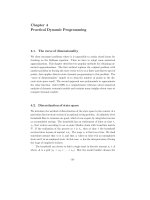
The graphical construction of the offer curve is illustrated in Fig. 9.2.1. We
trace it out by varying α
i
in the household’s problem and reading tangency
points between the household’s indifference curve and the budget line. The
resulting locus depends on the endowment vector and lies above the indifference
curve through the endowment vector. By construction the following property is
also true: at the intersection between the offer curve and a straight line through
the endowment point, the straight line is tangent to an indifference curve.
4
4
Given our assumptions on preferences and endowments, the conscientious
reader will find Fig. 9.2.1 deceptive because the offer curve appears to fail to
intersect the feasibility line at c
t
t
= c

t
t+1
, i.e., Equilibrium H above. Our excuse
for the deception is the expositional clarity that we gain when we introduce
additional objects in the graphs.
Time-0 trading 263
Offer curve
Feasibility line
to the endowment
corresponding
Indifference curve
c
t
t+1
c
t-1
t
y
t
t
y
t
t+1
c
t
t
,
Figure 9.2.1: The offer curve and feasibility line.
Following Gale (1973), we can use the offer curve and a straight line de-
picting feasibility in the (c

i
i
,c
i−1
i
) plane to construct a machine for computing
equilibrium allocations and prices. In particular, we can use the following pair
of difference equations to solve for an equilibrium allocation. For i ≥ 1, the
equations are
5
ψ(c
i
i
,c
i
i+1
)=0, (9.2.6a)
c
i
i
+ c
i−1
i
= y
i
i
+ y
i−1
i
. (9.2.6b)

After the allocation has been computed, the equilibrium price system can be
computed from
q
0
i
= u

(c
i
i
)
for all i ≥ 1.
5
By imposing equation (9.2.6b) with equality, we are implicitly possibly
including a giveaway program to the initial old.
264 Overlapping Generations Models
9.2.4. Computing equilibria
Example 1 Gale’s equilibrium computation machine: A procedure for con-
structing an equilibrium is illustrated in Fig. 9.2.2, which reproduces a version
of a graph of David Gale (1973). Start with a proposed c
1
1
, a time-1 allocation
to the initial young. Then use the feasibility line to find the maximal feasible
value for c
1
1
, the time-1 allocation to the initial old. In the Arrow-Debreu equi-
librium, the allocation to the initial old will be less than this maximal value, so
that some of the time 1 good is thrown away. The reason for this is that the

budget constraint of the initial old, q
0
1
(c
0
1
−y
0
1
) ≤ 0, implies that c
0
1
= y
0
1
.
6
The
candidate time-1 allocation is thus feasible, but the time-1 young will choose
c
1
1
only if the price α
1
is such that (c
1
2
,c
1
1

) lies on the offer curve. Therefore, we
choose c
1
2
from the point on the offer curve that cuts a vertical line through c
1
1
.
Then we proceed to find c
2
2
from the intersection of a horizontal line through
c
1
2
and the feasibility line. We continue recursively in this way, choosing c
i
i
as
the intersection of the feasibility line with a horizontal line through c
i−1
i
,then
choosing c
i
i+1
as the intersection of a vertical line through c
i
i
and the offer curve.

We can construct a sequence of α
i
’s from the slope of a straight line through
the endowment point and the sequence of (c
i
i
,c
i
i+1
) pairs that lie on the offer
curve.
If the offer curve has the shape drawn in Fig. 9.2.2, any c
1
1
between the
upper and lower intersections of the offer curve and the feasibility line is an equi-
librium setting of c
1
1
.Eachsuchc
1
1
is associated with a distinct allocation and
α
i
sequence, all but one of them converging to the low-interest-rate stationary
equilibrium allocation and interest rate.
Example 2 Endowment at +∞: Take the preference and endowment structure
of the previous example and modify only one feature. Change the endowment of
the initial old to be y

0
1
= >0 and “δ>0 units of consumption at t =+∞,”
by which we mean that we take

t
q
0
t
y
0
t
= q
0
1
 + δ lim
t→∞
q
0
t
.
It is easy to verify that the only competitive equilibrium of the economy with
this specification of endowments has q
0
t
=1∀t ≥ 1, and thus α
t
=1∀t ≥ 1.
6
Soon we shall discuss another market structure that avoids throwing away

any of the initial endowment by augmenting the endowment of the initial old
with a particular zero-dividend infinitely durable asset.
Time-0 trading 265
Offer curve
Feasibility line
c
t
t+1
c
t-1
t
y
t
t
cc
c
c
c
y
t
t+1
1
1
2
2
2
3
2
1
0

1
,
c
t
t
Figure 9.2.2: A nonstationary equilibrium allocation.
The reason is that all the “low-interest-rate” equilibria that we have described
would assign an infinite value to the endowment of the initial old. Confronted
with such prices, the initial old would demand unbounded consumption. That
is not feasible. Therefore, such a price system cannot be an equilibrium.
Example 3 A Lucas tree: Take the preference and endowment structure to
be the same as example 1 and modify only one feature. Endow the initial old
with a “Lucas tree,” namely, a claim to a constant stream of d>0 units of
consumption for each t ≥ 1.
7
Thus, the budget constraint of the initial old
person now becomes
q
0
1
c
0
1
= d
∞

t=1
q
0
t

+ q
0
1
y
0
1
.
The offer curve of each young agent remains as before, but now the feasibility
line is
c
i
i
+ c
i−1
i
= y
i
i
+ y
i−1
i
+ d
for all i ≥ 1. Note that young agents are endowed below the feasibility line.
From Fig. 9.2.3, it seems that there are two candidates for stationary equilibria,
7
This is a version of an example of Brock (1990).
266 Overlapping Generations Models
one with constant α<1, another with constant α>1. The one with α<1
is associated with the steeper budget line in Fig. 9.2.3 However, the candidate
stationary equilibrium with α>1 cannot be an equilibrium for a reason similar

to that encountered in example 2. At the price system associated with an
α>1, the wealth of the initial old would be unbounded, which would prompt
them to consume an unbounded amount, which is not feasible. This argument
rules out not only the stationary α>1 equilibrium but also all nonstationary
candidate equilibria that converge to that constant α . Therefore, there is a
unique equilibrium; it is stationary and has α<1.
Unique equilibrium
Feasibility line
Offer curve
c
t
t+1
c
t-1
t
y
t
t+1
without tree
Feasibility line
with tree
y
t
t
Not an equilibrium
(R>1)
R>1
R<1
dividend
,

c
t
t
Figure 9.2.3: Unique equilibrium with a fixed-dividend as-
set.
If we interpret the gross rate of return on the tree as α
−1
=
p+d
p
,where
p =

∞
t=1
q
0
t
d, we can compute that p =
d
R−1
where R = α
−1
.Herep is the
price of the Lucas tree.
In terms of the logarithmic preference example, the difference equation
(9.2.9) becomes modified to
α
i
=

1+2d

−

−1
− 1
α
i−1
. (9.2.7)
Time-0 trading 267
Example 4 Government expenditures: Take the preferences and endowments
to be as in example 1 again, but now alter the feasibility condition to be
c
i
i
+ c
i−1
i
+ g = y
i
i
+ y
i−1
i
for all i ≥ 1whereg>0 is a positive level of government purchases. The
“clearing house” is now looking for an equilibrium price vector such that this
feasibility constraint is satisfied. We assume that government purchases do
not give utility. The offer curve and the feasibility line look as in Fig. 9.2.4.
Notice that the endowment point (y
i

i
,y
i
i+1
) lies outside the relevant feasibility
line. Formally, this graph looks like example 3, but with a “negative dividend
d.” Now there are two stationary equilibria with α>1, and a continuum of
equilibria converging to the higher α equilibrium (the one with the lower slope
α
−1
of the associated budget line). Equilibria with α>1 cannot be ruled out
by the argument in example 3 because no one’s endowment sequence receives
infinite value when α>1.
Later, we shall interpret this example as one in which a government finances
a constant deficit either by money creation or by borrowing at a negative real
net interest rate. We shall discuss this and other examples in a setting with
sequential trading.
Example 5 Log utility: Suppose that u(c)=lnc and that the endowment is
described by equations (9.2.4). Then the offer curve is given by the recursive
formulas c
i
i
= .5(1 −  + α
i
),c
i
i+1
= α
−1
i

c
i
i
.Letα
i
be the gross rate of return
facing the young at i. Feasibility at i and the offer curves then imply
1
2α
i−1
(1 −  + α
i−1
)+.5(1 − + α
i
)=1. (9.2.8)
This implies the difference equation
α
i
= 
−1
−

−1
− 1
α
i−1
. (9.2.9)
See Fig. 9.2.2. An equilibrium α
i
sequence must satisfy equation (9.2.8) and

have α
i
> 0 for all i.Evidently,α
i
=1foralli ≥ 1 is an equilibrium
α sequence. So is any α
i
sequence satisfying equation (9.2.8) and α
1
≥ 1;
α
1
< 1 will not work because equation (9.2.8) implies that the tail of {α
i
} is
an unbounded negative sequence. The limiting value of α
i
for any α
1
> 1is
268 Overlapping Generations Models
c
t
t+1
c
t-1
t
y
t
t+1

y
t
t
without government spendings
Offer curve
Feasibility line
government
spendings
spendings
government
with
Feasibility line
(low inflation)
equilibrium
High interest rate
Low interest rate
equilibrium
(high inflation)
,
c
t
t
Figure 9.2.4: Equilibria with debt- or money-financed gov-
ernment deficit finance.
1−

= u

()/u


(1 −), which is the interest factor associated with the stationary
autarkic equilibrium. Notice that Fig. 9.2.2 suggests that the stationary α
i
=1
equilibrium is not stable, while the autarkic equilibrium is.
9.3. Sequential trading
We now alter the trading arrangement to bring us into line with standard presen-
tations of the overlapping generations model. We abandon the time-0, complete
market trading arrangement and replace it with sequential trading in which a
durable asset, either government debt or money or claims on a Lucas tree, are
passed from old to young. Some cross-generation transfers occur with voluntary
exchanges while others are engineered by government tax and transfer programs.
Money 269
9.4. Money
In Samuelson’s (1958) version of the model, trading occurs sequentially through
a medium of exchange, an inconvertible (or “fiat”) currency. In Samuelson’s
model, the preferences and endowments are as described previously, with one
important additional component of the endowment. At date t = 1, old agents
are endowed in the aggregate with M>0 units of intrinsically worthless cur-
rency. No one has promised to redeem the currency for goods. The currency
is not “backed” by any government promise to redeem it for goods. But as
Samuelson showed, there can exist a system of expectations that will make the
currency be valued. Currency will be valued today if people expect it to be
valued tomorrow. Samuelson thus envisioned a situation in which currency is
backed by expectations without promises.
For each date t ≥ 1, young agents purchase m
i
t
units of currency at a price
of 1/p

t
units of the time-t consumption good. Here p
t
≥ 0isthetime-t price
level. At each t ≥ 1, each old agent exchanges his holdings of currency for the
time-t consumption good. The budget constraints of a young agent born in
period i ≥ 1are
c
i
i
+
m
i
i
p
i
≤ y
i
i
, (9.4.1)
c
i
i+1
≤
m
i
i
p
i+1
+ y

i
i+1
, (9.4.2)
m
i
i
≥ 0. (9.4.3)
If m
i
i
≥ 0, inequalities (9.4.1) and (9.4.2) imply
c
i
i
+ c
i
i+1

p
i+1
p
i

≤ y
i
i
+ y
i
i+1


p
i+1
p
i

. (9.4.4)
Provided that we set
p
i+1
p
i
= α
i
=
q
0
i+1
q
0
i
,
this budget set is identical with equation (9.2.1).
We use the following definitions:
Definition: A nominal price sequence is a positive sequence {p
i
}
i≥1
.
270 Overlapping Generations Models
Definition: An equilibrium with valued fiat money is a feasible allocation

and a nominal price sequence with p
t
< +∞ for all t such that given the price
sequence, the allocation solves the household’s problem for each i ≥ 1.
The qualification that p
t
< +∞ for all t means that fiat money is valued.
9.4.1. Computing more equilibria
Summarize the household’s optimal decisions with a saving function
y
i
i
− c
i
i
= s(α
i
; y
i
i
,y
i
i+1
). (9.4.5)
Then the equilibrium conditions for the model are
M
p
i
= s(α
i

; y
i
i
,y
i
i+1
)(9.4.6a)
α
i
=
p
i+1
p
i
, (9.4.6b)
where it is understood that c
i
i+1
= y
i
i+1
+
M
p
i+1
. To compute an equilibrium, we
solve the difference equations (9.4.6) for {p
i
}
∞

i=1
, then get the allocation from
the household’s budget constraints evaluated at equality at the equilibrium level
of real balances. As an example, suppose that u(c)=ln(c), and that (y
i
i
,y
i
i+1
)=
(w
1
,w
2
)withw
1
>w
2
. The saving function is s(α
i
)=.5(w
1
− α
i
w
2
). Then
equation (9.4.6a) becomes
.5(w
1

− w
2
p
t+1
p
t
)=
M
p
t
or
p
t
=2M/w
1
+

w
2
w
1

p
t+1
. (9.4.7)
This is a difference equation whose solutions with a positive price level are
p
t
=
2M

w
1
(1 −
w
2
w
1
)
+ c

w
1
w
2

t
, (9.4.8)
for any scalar c>0.
8
The solution for c = 0 is the unique stationary solution.
The solutions with c>0 have uniformly higher price levels than the c =0
solution, and have the value of currency going to zero.
8
See the appendix to chapter 2.
Money 271
9.4.2. Equivalence of equilibria
We briefly look back at the equilibria with time-0 trading and note that the
equilibrium allocations are the same under time-0 and sequential trading. Thus,
the following proposition asserts that with an adjustment to the endowment and
the consumption allocated to the initial old, a competitive equilibrium allocation

with time-0 trading is an equilibrium allocation in the fiat money economy (with
sequential trading).
Proposition: Let c
i
denote a competitive equilibrium allocation (with time-
0 trading) and suppose that it satisfies
c
1
1
<y
1
1
. Then there exists an equilibrium
(with sequential trading) of the monetary economy with allocation that satisfies
c
i
i
= c
i
i
,c
i
i+1
= c
i
i+1
for i ≥ 1.
Proof: Take the competitive equilibrium allocation and price system and
form α
i

= q
0
i+1
/q
0
i
.Setm
i
i
/p
i
= y
i
i
− c
i
i
.Setm
i
i
= M for all i ≥ 1, and
determine p
1
from
M
p
1
= y
1
1

− c
1
1
. This last equation determines a positive
initial price level p
1
provided that y
1
1
− c
1
1
> 0. Determine subsequent price
levels from p
i+1
= α
i
p
i
. Determine the allocation to the initial old from c
0
1
=
y
0
1
+
M
p
1

= y
0
1
+(y
1
1
− c
1
1
).
In the monetary equilibrium, time-t real balances equal the per capita
savings of the young and the per capita dissavings of the old. To be in a
monetary equilibrium, both quantities must be positive for all t ≥ 1.
A converse of the proposition is true.
Proposition: Let c
i
be an equilibrium allocation for the fiat money econ-
omy. Then there is a competitive equilibrium with time 0 trading with the same
allocation, provided that the endowment of the initial old is augmented with a
particular transfer from the “clearing house.”
To verify this proposition, we have to construct the required transfer from
the clearing house to the initial old. Evidently, it is y
1
1
− c
1
1
. Weinvitethe
reader to complete the proof.
272 Overlapping Generations Models

9.5. Deficit finance
For the rest of this chapter, we shall assume sequential trading. With sequential
trading of fiat currency, this section reinterprets one of our earlier examples with
time-0 trading, the example with government spending.
Consider the following overlapping generations model: The population is
constant. At each date t ≥ 1, N identical young agents are endowed with
(y
t
t
,y
t
t+1
)=(w
1
,w
2
), where w
1
>w
2
> 0. A government levies lump-sum
taxes of τ
1
on each young agent and τ
2
on each old agent alive at each t ≥ 1.
There are N old people at time 1 each of whom is endowed with w
2
units
of the consumption good and M

0
> 0 units of inconvertible perfectly durable
fiat currency. The initial old have utility function c
0
1
. The young have utility
function u(c
t
t
)+u(c
t
t+1
). For each date t ≥ 1 the government augments the
currency supply according to
M
t
− M
t−1
= p
t
(g −τ
1
− τ
2
), (9.5.1)
where g is a constant stream of government expenditures per capita and 0 <
p
t
≤ +∞ is the price level. If p
t

=+∞,weintendthatequation(9.5.1) be
interpreted as
g = τ
1
+ τ
2
. (9.5.2)
For each t ≥ 1, each young person’s behavior is summarized by
s
t
= f (R
t
; τ
1
,τ
2
) = arg max
s≥0
[u(w
1
− τ
1
− s)+u(w
2
− τ
2
+ R
t
s)] . (9.5.3)
Definition: An equilibrium with valued fiat currency is a pair of positive

sequences {M
t
,p
t
} such that (a) given the price level sequence, M
t
/p
t
= f (R
t
)
(the dependence on τ
1
,τ
2
being understood); (b) R
t
= p
t
/p
t+1
; and (c) the
government budget constraint (9.5.1) is satisfied for all t ≥ 1.
The condition f (R
t
)=M
t
/p
t
canbewrittenasf(R

t
)=M
t−1
/p
t
+(M
t
−
M
t−1
)/p
t
. The left side is the savings of the young. The first term on the right
side is the dissaving of the old (the real value of currency that they exchange
for time-t consumption). The second term on the right is the dissaving of the
government (its deficit), which is the real value of the additional currency that
the government prints at t and uses to purchase time-t goods from the young.
Deficit finance 273
To compute an equilibrium, define d = g − τ
1
− τ
2
and write equation
(9.5.1) as
M
t
p
t
=
M

t−1
p
t−1
p
t−1
p
t
+ d
for t ≥ 2and
M
1
p
1
=
M
0
p
1
+ d
for t = 1 . Substitute M
t
/p
t
= f (R
t
) into these equations to get
f(R
t
)=f(R
t−1

)R
t−1
+ d (9.5.4a)
for t ≥ 2and
f(R
1
)=
M
0
p
1
+ d. (9.5.4b)
Given p
1
, which determines an initial R
1
by means of equation (9.5.4b),
equations (9.5.4) form an autonomous difference equation in R
t
.Thissystem
can be solved using Fig. 9.2.4.
9.5.1. Steady states and the Laffer curve
Let’s seek a stationary solution of equations (9.5.4), a quest that is rendered
reasonable by the fact that f (R
t
) is time invariant (because the endowment and
the tax patterns as well as the government deficit d are time invariant). Guess
that R
t
= R for t ≥ 1. Then equations (9.5.4) become

f(R)(1 −R)=d, (9.5.5a)
f(R)=
M
0
p
1
+ d. (9.5.5b)
For example, suppose that u(c)=ln(c). Then f (R)=
w
1
−τ
1
2
−
w
2
−τ
2
2R
.We
have graphed f(R)(1 − R) against d in Fig. 9.5.1. Notice that if there is one
solution for equation (9.5.5a), then there are at least two.
Here (1−R) can be interpreted as a tax rate on real balances, and f(R)(1−
R) is a Laffer curve for the inflation tax rate. The high-return (low-tax) R =
R
is associated with the good Laffer curve stationary equilibrium, and the low-
return (high-tax) R = R
comes with the bad Laffer curve stationary equilibrium.
Once R is determined, we can determine p
1

from equation (9.5.5b).
274 Overlapping Generations Models
ReciprocalHigh inflation
equilibrium
(low interest rate)
Low inflation
equilibrium
(hi
g
h interest rate)
government
spendings
Seigneuriage earnings
of the gross inflation rate
Figure 9.5.1: The Laffer curve in revenues from the inflation
tax.
Fig. 9.5.1 is isomorphic with Fig. 9.2.4. The saving rate function f(R)can
be deduced from the offer curve. Thus, a version of Fig. 9.2.4 can be used to
solve the difference equation (9.5.4a) graphically. If we do so, we discover a
continuum of nonstationary solutions of equation (9.5.4a), all but one of which
have R
t
→ R as t →∞. Thus, the bad Laffer curve equilibrium is stable.
The stability of the bad Laffer curve equilibrium arises under perfect fore-
sight dynamics. Bruno and Fischer (1990) and Marcet and Sargent (1989) an-
alyze how the system behaves under two different types of adaptive dynamics.
They find that either under a crude form of adaptive expectations or under a
least squares learning scheme, R
t
converges to R. This finding is comforting be-

cause the comparative dynamics are more plausible at
R (larger deficits bring
higher inflation). Furthermore, Marimon and Sunder (1993) present experi-
mental evidence pointing toward the selection made by the adaptive dynamics.
Marcet and Nicolini (1999) build an adaptive model of several Latin American
hyperinflations that rests on this selection.
Equivalent setups 275
9.6. Equivalent setups
This section describes some alternative asset structures and trading arrange-
ments that support the same equilibrium allocation. We take a model with
a government deficit and show how it can be supported with sequential trad-
ing in government-indexed bonds, sequential trading in fiat currency, or time-0
trading in Arrow-Debreu dated securities.
9.6.1. The economy
Consider an overlapping generations economy with one agent born at each t ≥ 1
and an initial old person at t = 1. Young agents born at date t have endowment
pattern (y
t
t
,y
t
t+1
) and the utility function described earlier. The initial old
person is endowed with M
0
> 0 units of unbacked currency and y
0
1
units of the
consumption good. There is a stream of per-young-person government purchases

{g
t
}.
Definition: An equilibrium with money financed government deficits is a
sequence {M
t
,p
t
}
∞
t=1
with 0 <p
t
< +∞ and M
t
> 0 that satisfies (a) given
{p
t
},
M
t
=argmax
˜
M≥0

u(y
t
t
−
˜

M/p
t
)+u(y
t
t+1
+
˜
M/p
t+1
)

;(9.6.1a)
and (b)
M
t
− M
t−1
= p
t
g
t
. (9.6.1b)
Now consider a version of the same economy in which there is no currency
but rather indexed government bonds. The demographics and endowments are
identical with the preceding economy, but now each initial old person is endowed
with B
1
units of a maturing bond, denominated in units of time-1 consumption
good. In period t, the government sells new one-period bonds to the young to
finance its purchases g

t
of time-t goods and to pay off the one-period debt
falling due at time t.LetR
t
> 0 be the gross real one-period rate of return on
government debt between t and t +1.
Definition: An equilibrium with bond-financed government deficits is a
sequence {B
t+1
,R
t
}
∞
t=1
that satisfies (a) given {R
t
},
B
t+1
=argmax
˜
B
[u(y
t
t
−
˜
B/R
t
)+u(y

t
t+1
+
˜
B)]; (9.6.2a)
276 Overlapping Generations Models
and (b)
B
t+1
/R
t
= B
t
+ g
t
, (9.6.2b)
with B
1
≥ 0given.
These two types of equilibria are isomorphic in the following sense: Take
an equilibrium of the economy with money-financed deficits and transform it
into an equilibrium of the economy with bond-financed deficits as follows: set
B
t
= M
t−1
/p
t
,R
t

= p
t
/p
t+1
. It can be verified directly that these settings
of bonds and interest rates, together with the original consumption allocation,
form an equilibrium of the economy with bond-financed deficits.
Each of these two types of equilibria is evidently also isomorphic to the
following equilibrium formulated with time-0 markets:
Definition: Let B
g
1
represent claims to time-1 consumption owed by the
government to the old at time 1. An equilibrium with time-0 trading is an
initial level of government debt B
g
1
,apricesystem{q
0
t
}
∞
t=1
, and a sequence
{s
t
}
∞
t=1
such that (a) given the price system,

s
t
=argmax
˜s

u(y
t
t
− ˜s)+u

y
t
t+1
+

q
0
t
q
0
t+1

˜s

;
and (b)
q
0
1
B

g
1
+
∞

t=1
q
0
t
g
t
=0. (9.6.3)
Condition b is the Arrow-Debreu version of the government budget con-
straint. Condition a is the optimality condition for the intertemporal consump-
tion decision of the young of generation t.
The government budget constraint in condition b can be represented recur-
sively as
q
0
t+1
B
g
t+1
= q
0
t
B
g
t
+ q

0
t
g
t
. (9.6.4)
If we solve equation (9.6.4) forward and impose lim
T →∞
q
0
t+T
B
g
t+T
=0,we
obtain the budget constraint (9.6.3) for t = 1. Condition (9.6.3) makes it
evident that when

∞
t=1
q
0
t
g
t
> 0, B
g
1
< 0, so that the government has negative
net worth. This negative net worth corresponds to the unbacked claims that
the market nevertheless values in the sequential trading version of the model.

Equivalent setups 277
9.6.2. Growth
It is easy to extend these models to the case in which there is growth in the
population. Let there be N
t
= nN
t−1
identical young people at time t,with
n>0. For example, consider the economy with money-financed deficits. The
total money supply is N
t
M
t
, and the government budget constraint is
N
t
M
t
− N
t−1
M
t−1
= N
t
p
t
g,
where g is per-young-person government purchases. Dividing both sides of the
budget constraint by N
t

and rearranging gives
M
t
p
t+1
p
t+1
p
t
= n
−1
M
t−1
p
t
+ g. (9.6.5)
This equation replaces equation (9.6.1b) in the definition of an equilibrium with
money-financed deficits. (Note that in a steady state R = n is the high-interest-
rate equilibrium.) Similarly, in the economy with bond-financed deficits, the
government budget constraint would become
B
t+1
R
t
= n
−1
B
t
+ g
t

.
It is also easy to modify things to permit the government to tax young and
old people at t. In that case, with government bond finance the government
budget constraint becomes
B
t+1
R
t
= n
−1
B
t
+ g
t
− τ
t
t
− n
−1
τ
t−1
t
,
where τ
s
t
is the time t tax on a person born in period s.
278 Overlapping Generations Models
9.7. Optimality and the existence of monetary equilibria
Wallace (1980) discusses the connection between nonoptimality of the equilib-

rium without valued money and existence of monetary equilibria. Abstracting
from his assumption of a storage technology, we study how the arguments ap-
ply to a pure endowment economy. The environment is as follows. At any
date t, the population consists of N
t
young agents and N
t−1
old agents where
N
t
= nN
t−1
with n>0. Each young person is endowed with y
1
> 0 goods, and
an old person receives the endowment y
2
> 0. Preferences of a young agent at
time t are given by the utility function u(c
t
t
,c
t
t+1
) which is twice differentiable
with indifference curves that are convex to the origin. The two goods in the
utility function are normal goods, and
θ(c
1
,c

2
) ≡ u
1
(c
1
,c
2
)/u
2
(c
1
,c
2
),
the marginal rate of substitution function, approaches infinity as c
2
/c
1
ap-
proaches infinity and approaches zero as c
2
/c
1
approaches zero. The welfare
of the initial old agents at time 1 is strictly increasing in c
0
1
,andeachoneof
them is endowed with y
2

goods and m
0
0
> 0 units of fiat money. Thus, the
beginning-of-period aggregate nominal money balances in the initial period 1
are M
0
= N
0
m
0
0
.
For all t ≥ 1, M
t
, the post-transfer time t stock of fiat money, obeys
M
t
= zM
t−1
with z>0. The time t transfer (or tax), (z −1)M
t−1
, is divided
equally at time t among the N
t−1
members of the current old generation. The
transfers (or taxes) are fully anticipated and are viewed as lump-sum: they do
not depend on consumption and saving behavior. The budget constraints of a
young agent born in period t are
c

t
t
+
m
t
t
p
t
≤ y
1
, (9.7.1)
c
t
t+1
≤ y
2
+
m
t
t
p
t+1
+
(z − 1)
N
t
M
t
p
t+1

, (9.7.2)
m
t
t
≥ 0, (9.7.3)
where p
t
> 0isthetimet price level. In a nonmonetary equilibrium, the price
level is infinite so the real value of both money holdings and transfers are zero.
Since all members in a generation are identical, the nonmonetary equilibrium is
autarky with a marginal rate of substitution equal to
θ
aut
≡
u
1
(y
1
,y
2
)
u
2
(y
1
,y
2
)
.
Optimality and the existence of monetary equilibria 279

We ask two questions about this economy. Under what circumstances does a
monetary equilibrium exist? And, when it exists, under what circumstances
does it improve matters?
Let ˆm
t
denote the equilibrium real money balances of a young agent at time
t,ˆm
t
≡ M
t
/(N
t
p
t
). Substitution of equilibrium money holdings into budget
constraints (9.7.1) and (9.7.2) at equality yield c
t
t
= y
1
− ˆm
t
and c
t
t+1
=
y
2
+ n ˆm
t+1

. In a monetary equilibrium, ˆm
t
> 0 for all t and the marginal rate
of substitution θ(c
t
t
,c
t
t+1
)satisfies
θ(y
1
− ˆm
t
,y
2
+ n ˆm
t+1
)=
p
t
p
t+1
>θ
aut
, ∀t ≥ 1. (9.7.4)
The equality part of (9.7.4) is the first-order condition for money holdings of an
agent born in period t evaluated at the equilibrium allocation. Since c
t
t

<y
1
and c
t
t+1
>y
2
in a monetary equilibrium, the inequality in (9.7.4) follows from
the assumption that the two goods in the utility function are normal goods.
Another useful characterization of the equilibrium rate of return on money,
p
t
/p
t+1
, can be obtained as follows. By the rule generating M
t
and the equi-
librium condition M
t
/p
t
= N
t
ˆm
t
, we have for all t,
p
t
p
t+1

=
M
t+1
zM
t
p
t
p
t+1
=
N
t+1
ˆm
t+1
zN
t
ˆm
t
=
n
z
ˆm
t+1
ˆm
t
. (9.7.5)
We are now ready to address our first question, under what circumstances does
a monetary equilibrium exist?
Proposition: θ
aut

z<nis necessary and sufficient for the existence of at
least one monetary equilibrium.
Proof: We first establish necessity. Suppose to the contrary that there is a
monetary equilibrium and θ
aut
z/n ≥ 1. Then, by the inequality part of (9.7.4)
and expression (9.7.5),wehaveforallt,
ˆm
t+1
ˆm
t
>
zθ
aut
n
≥ 1. (9.7.6)
If zθ
aut
/n > 1, one plus the net growth rate of ˆm
t
is bounded uniformly above
one and, hence, the sequence {ˆm
t
} is unbounded which is inconsistent with
an equilibrium because real money balances per capita cannot exceed the en-
dowment y
1
of a young agent. If zθ
aut
/n = 1, the strictly increasing sequence

280 Overlapping Generations Models
{ˆm
t
} in (9.7.6) might not be unbounded but converge to some constant ˆm
∞
.
According to (9.7.4) and (9.7.5), the marginal rate of substitution will then
converge to n/z which by assumption is now equal to θ
aut
, the marginal rate of
substitution in autarky. Thus, real balances must be zero in the limit which con-
tradicts the existence of a strictly increasing sequence of positive real balances
in (9.7.6) .
To show sufficiency, we prove the existence of a unique equilibrium with
constant per-capita real money balances when θ
aut
z<n. Substitute our can-
didate equilibrium, ˆm
t
=ˆm
t+1
≡ ˆm,into(9.7.4) and (9.7.5), which yields two
equilibrium conditions,
θ(y
1
− ˆm, y
2
+ n ˆm)=
n
z

>θ
aut
.
The inequality part is satisfied under the parameter restriction of the proposi-
tion, and we only have to show the existence of ˆm ∈ [0,y
1
] that satisfies the
equality part. But the existence (and uniqueness) of such a ˆm is trivial. Note
that the marginal rate of substitution on the left side of the equality is equal
to θ
aut
when ˆm = 0. Next, our assumptions on preferences imply that the
marginal rate of substitution is strictly increasing in ˆm, and approaches infinity
when ˆm approaches y
1
.
The stationary monetary equilibrium in the proof will be referred to as the
ˆm equilibrium. In general, there are other nonstationary monetary equilibria
when the parameter condition of the proposition is satisfied. For example, in
the case of logarithmic preferences and a constant population, recall the con-
tinuum of equilibria indexed by the scalar c>0 in expression (9.4.8). But
here we choose to focus solely on the stationary ˆm equilibrium, and its welfare
implications. The ˆm equilibrium will be compared to other feasible allocations
using the Pareto criterion. Evidently, an allocation C = {c
0
1
;(c
t
t
,c

t
t+1
),t≥ 1} is
feasible if
N
t
c
t
t
+ N
t−1
c
t−1
t
≤ N
t
y
1
+ N
t−1
y
2
, ∀t ≥ 1,
or, equivalently,
nc
t
t
+ c
t−1
t

≤ ny
1
+ y
2
, ∀t ≥ 1. (9.7.7)
The definition of Pareto optimality is:
Optimality and the existence of monetary equilibria 281
Definition: A feasible allocation C is Pareto optimal if there is no other
feasible allocation
˜
C such that
˜c
0
1
≥ c
0
1
,
u(˜c
t
t
, ˜c
t
t+1
) ≥ u(c
t
t
,c
t
t+1

), ∀t ≥ 1,
and at least one of these weak inequalities holds with strict inequality.
We first examine under what circumstances the nonmonetary equilibrium
(autarky) is Pareto optimal.
Proposition: θ
aut
≥ n is necessary and sufficient for the optimality of the
nonmonetary equilibrium (autarky).
Proof: To establish sufficiency, suppose to the contrary that there exists
another feasible allocation
˜
C that is Pareto superior to autarky and θ
aut
≥ n.
Without loss of generality, assume that the allocation
˜
C satisfies (9.7.7) with
equality. (Given an allocation that is Pareto superior to autarky but that does
not satisfy (9.7.7), one can easily construct another allocation that is Pareto
superior to the given allocation, and hence to autarky.) Let period t be the first
period when this alternative allocation
˜
C differs from the autarkic allocation.
The requirement that the old generation in this period is not made worse off,
˜c
t−1
t
≥ y
2
, implies that the first perturbation from the autarkic allocation must

be ˜c
t
t
<y
1
with the subsequent implication that ˜c
t
t+1
>y
2
. It follows that
the consumption of young agents at time t + 1 must also fall below y
1
,andwe
define

t+1
≡ y
1
− ˜c
t+1
t+1
> 0. (9.7.8)
Now, given ˜c
t+1
t+1
, we compute the smallest number c
t+1
t+2
that satisfies

u(˜c
t+1
t+1
,c
t+1
t+2
) ≥ u(y
1
,y
2
).
Let
c
t+1
t+2
be the solution to this problem. Since the allocation
˜
C is Pareto
superior to autarky, we have ˜c
t+1
t+2
≥ c
t+1
t+2
. Before using this inequality, though,
we want to derive a convenient expression for
c
t+1
t+2
.

Consider the indifference curve of u(c
1
,c
2
) that yields a fixed utility equal
to u(y
1
,y
2
). In general, along an indifference curve, c
2
= h(c
1
)whereh

=
282 Overlapping Generations Models
−u
1
/u
2
= −θ and h

> 0. Therefore, applying the intermediate value theorem
to h,wehave
h(c
1
)=h(y
1
)+(y

1
− c
1
)[−h

(y
1
)+f(y
1
− c
1
)], (9.7.9)
where the function f is strictly increasing and f(0) = 0.
Now since (˜c
t+1
t+1
, c
t+1
t+2
)and(y
1
,y
2
) are on the same indifference curve, we
may use (9.7.8) and (9.7.9) to write
c
t+1
t+2
= y
2

+ 
t+1
[θ
aut
+ f(
t+1
)],
and after invoking ˜c
t+1
t+2
≥ c
t+1
t+2
,wehave
˜c
t+1
t+2
− y
2
≥ 
t+1
[θ
aut
+ f(
t+1
)]. (9.7.10)
Since
˜
C satisfies (9.7.7) at equality, we also have


t+2
≡ y
1
− ˜c
t+2
t+2
=
˜c
t+1
t+2
− y
2
n
. (9.7.11)
Substitution of (9.7.10) into (9.7.11) yields

t+2
≥ 
t+1
θ
aut
+ f(
t+1
)
n
>
t+1
,
(9.7.12)
where the strict inequality follows from θ

aut
≥ n and f (
t+1
) > 0 (implied by

t+1
> 0). Continuing these computations of successive values of 
t+k
yields

t+k
≥ 
t+1
k−1

j=1
θ
aut
+ f(
t+j
)
n
>
t+1

θ
aut
+ f(
t+1
)

n

k−1
, for k>2,
where the strict inequality follows from the fact that {
t+j
} is a strictly increas-
ing sequence. Thus the  sequence is bounded below by a strictly increasing
exponential and hence is unbounded. But such an unbounded sequence violates
feasibility because  cannot exceed the endowment y
1
of a young agent, it fol-
lows that we can rule out the existence of a Pareto superior allocation
˜
C ,and
conclude that θ
aut
≥ n is a sufficient condition for the optimality of autarky.
To establish necessity, we prove the existence of an alternative feasible al-
location
ˆ
C that is Pareto superior to autarky when θ
aut
<n. First, pick an
>0 sufficiently small so that
θ
aut
+ f() ≤ n, (9.7.13)