Recursive macroeconomic theory, Thomas Sargent 2nd Ed - Chapter 25 pps

Chapter 25
Credit and Currency
25.1. Credit and currency with long-lived agents
This chapter describes Townsend’s (1980) turnpike model of money and puts it
to work. The model uses a particular pattern of heterogeneity of endowments
and locations to create a demand for currency. The model is more primitive than
the shopping time model of chapter 24. As with the overlapping generations
model, the turnpike model starts from a setting in which diverse intertemporal
endowment patterns across agents prompt borrowing and lending. If something
prevents loan markets from operating, it is possible that an unbacked currency
can play a role in helping agents smooth their consumption over time. Following
Townsend, we shall eventually appeal to locational heterogeneity as the force
that causes loan markets to fail in this way.
The turnpike model can be viewed as a simplified version of the stochastic
model proposed by Truman Bewley (1980). We use the model to study a number
of interrelated issues and theories, including (1) a permanent income theory of
consumption, (2) a Ricardian doctrine that government borrowing and taxes
have equivalent economic effects, (3) some restrictions on the operation of private
loan markets needed in order that unbacked currency be valued, (4) a theory of
inflationary finance, (5) a theory of the optimal inflation rate and the optimal
behavior of the currency stock over time, (6) a “legal restrictions” theory of
inflationary finance, and (7) a theory of exchange rate indeterminacy.
1
1
Some of the analysis in this chapter follows Manuelli and Sargent (1992).
Also see Chatterjee and Corbae (1996) and Ireland (1994) for analyses of policies
within a turnpike environment.
– 897 –
898 Credit and Currency
25.2. Preferences and endowments
There is one consumption good. It cannot be produced or stored. The total

amount of goods available each period is constant at N .Thereare2N house-
holds, divided into equal numbers N of two types, according to their endowment
sequences. The two types of households, dubbed odd and even, have endowment
sequences
{y
o
t
}
∞
t=0
= {1, 0, 1, 0, },
{y
e
t
}
∞
t=0
= {0, 1, 0, 1, }.
Households of both types order consumption sequences {c
h
t
} according to the
common utility function
U =
∞

t=0
β
t
u(c

h
t
),
where β ∈ (0, 1), and u(·) is twice continuously differentiable, increasing and
strictly concave, and satisfies
lim
c↓0
u

(c)=+∞. (25.2.1)
25.3. Complete markets
Asabenchmark,westudyaversionofthe economy with complete markets.
Later we shall more or less arbitrarily shut down many of the markets to make
room for money.
Complete markets 899
25.3.1. A Pareto problem
Consider the following Pareto problem: Let θ ∈ [0, 1] be a weight indexing how
much a social planner likes odd agents. The problem is to choose consumption
sequences {c
o
t
,c
e
t
}
∞
t=0
to maximize
θ
∞


t=0
β
t
u(c
o
t
)+(1−θ)
∞

t=0
β
t
u(c
e
t
), (25.3.1)
subject to
c
e
t
+ c
o
t
=1,t≥ 0. (25.3.2)
The first-order conditions are
θu

(c
o

t
) − (1 −θ)u

(c
e
t
)=0.
Substituting the constraint (25.3.2) into this first-order condition and rearrang-
ing gives the condition
u

(c
o
t
)
u

(1 − c
o
t
)
=
1 −θ
θ
. (25.3.3)
Since the right side is independent of time, the left must be also, so that condition
(25.3.3) determines the one-parameter family of optimal allocations
c
o
t

= c
o
(θ),c
e
t
=1−c
o
(θ).
25.3.2. A complete markets equilibrium
A household takes the price sequence {q
0
t
} as given and chooses a consumption
sequence to maximize

∞
t=0
β
t
u(c
t
) subject to the budget constraint
∞

t=0
q
0
t
c
t

≤
∞

t=0
q
0
t
y
t
.
The household’s Lagrangian is
L =
∞

t=0
β
t
u(c
t
)+µ
∞

t=0
q
0
t
(y
t
− c
t

),
900 Credit and Currency
where µ is a nonnegative Lagrange multiplier. The first-order conditions for the
household’s problem are
β
t
u

(c
t
) ≤ µq
0
t
, =ifc
t
> 0.
Definition 1: A competitive equilibrium is a price sequence {q
o
t
}
∞
t=0
and an
allocation {c
o
t
,c
e
t
}

∞
t=0
that have the property that (a) given the price sequence,
the allocation solves the optimum problem of households of both types, and (b)
c
o
t
+ c
e
t
=1 forallt ≥ 0.
To find an equilibrium, we have to produce an allocation and a price system
for which we can verify that the first-order conditions of both households are
satisfied. We start with a guess inspired by the constant-consumption property
of the Pareto optimal allocation. We guess that c
o
t
= c
o
,c
e
t
= c
e
∀t, where
c
e
+ c
o
= 1. This guess and the first-order condition for the odd agents imply

q
0
t
=
β
t
u

(c
o
)
µ
o
,
or
q
0
t
= q
0
0
β
t
, (25.3.4)
where we are free to normalize by setting q
0
0
=1. For odd agents, the right side
of the budget constraint evaluated at the prices given in equation (25.3.4) is
then

1
1 −β
2
,
and for even households it is
β
1 −β
2
.
The left side of the budget constraint evaluated at these prices is
c
i
1 −β
,i= o, e.
For both of the budget constraints to be satisfied with equality we evidently
require that
c
o
=
1
β +1
c
e
=
β
β +1
.
(25.3.5)
Complete markets 901
The price system given by equation (25.3.4) and the constant over time alloca-

tions given by equations (25.3.5) are a competitive equilibrium.
Notice that the competitive equilibrium allocation corresponds to a particu-
lar Pareto optimal allocation.
25.3.3. Ricardian proposition
We temporarily add a government to the model. The government levies lump-
sum taxes on agents of type i = o, e at time t of τ
i
t
. The government uses the
proceeds to finance a constant level of government purchases of G ∈ (0, 1) each
period t.Consumeri’s budget constraint is
∞

t=0
q
0
t
c
i
t
≤
∞

t=0
q
0
t
(y
i
t

− τ
i
t
).
The government’s budget constraint is
∞

t=0
q
0
t
G =

i=o,e
∞

t=0
q
0
t
τ
i
t
.
We modify Definition 1 as follows:
Definition 2: A competitive equilibrium is a price sequence {q
0
t
}
∞

t=0
,atax
system { τ
o
t
,τ
e
t
}
∞
t=0
, and an allocation {c
o
t
,c
e
t
,G
t
}
∞
t=0
such that given the price
system and the tax system the following conditions hold: (a) the allocation
solves each consumer’s optimum problem, (b) the government budget constraint
is satisfied for all t ≥ 0, and (c) N(c
o
t
+ c
e

t
)+G
t
= N for all t ≥ 0.
Let the present value of the taxes imposed on consumer i be τ
i
≡

∞
t=0
q
0
t
τ
i
t
.
Then it is straightforward to verify that the equilibrium price system is still
equation (25.3.4) and that equilibrium allocations are
c
o
=
1
β +1
− τ
o
(1 − β)
c
e
=

β
β +1
− τ
e
(1 − β).
This equilibrium features a “Ricardian proposition”:
902 Credit and Currency
Ricardian Proposition: The equilibrium is invariant to changes in the
timing of tax collections that leave unaltered the present value of lump-sum
taxes assigned to each agent.
25.3.4. Loan market interpretation
Define total time-t tax collections as τ
t
=

i=o,e
τ
i
t
, and write the government’s
budget constraint as
(G
0
− τ
0
)=
∞

t=1
q

0
t
q
0
0
(τ
t
− G
t
) ≡ B
1
,
where B
1
can be interpreted as government debt issued at time 0 and due at
time 1. Notice that B
1
equals the present value of the future (i.e., from time 1
onward) government surpluses (τ
t
− G
t
). The government’s budget constraint
can also be represented as
q
0
0
q
0
1

(G
0
− τ
0
)+(G
1
− τ
1
)=
∞

t=2
q
0
t
q
0
1
(τ
t
− G
t
) ≡ B
2
,
or
R
1
B
1

+(G
1
− τ
1
)=B
2
,
where R
1
=
q
0
0
q
0
1
is the gross rate of return between time 0 and time 1, measured
in time-1 consumption goods per unit of time-0 consumption good. More gen-
erally, we can represent the government’s budget constraint by the sequence of
budget constraints
R
t
B
t
+(G
t
− τ
t
)=B
t+1

,t≥ 0,
subject to the boundary condition B
0
= 0. In the equilibrium computed here,
R
t
= β
−1
for all t ≥ 1.
Similar manipulations of consumers’ budget constraints can be used to ex-
press them in terms of sequences of one-period budget constraints. That no
opportunities are lost to the government or the consumers by representing the
budget sets in this way lies behind the following fact: the Arrow-Debreu allo-
cation in this economy can be implemented with a sequence of one-period loan
markets.
A monetary economy 903
In the following section, we shut down all loan markets, and also set govern-
ment expenditures G =0.
25.4. A monetary economy
We keep preferences and endowment patterns as they were in the preceding
economy, but we rule out all intertemporal trades achieved through borrowing
and lending or trading of future-dated consumptions. We replace complete
markets with a fiat money mechanism. At time 0, the government endows each
of the N even agents with M/N units of an unbacked or inconvertible currency.
Odd agents are initially endowed with zero units of the currency. Let p
t
be the
time-t price level, denominated in dollars per time-t consumption good. We
seek an equilibrium in which currency is valued (p
t

< +∞∀t ≥ 0)andinwhich
each period agents not endowed with goods pass currency to agents who are
endowed with goods. Contemporaneous exchanges of currency for goods are the
only exchanges that we, the model builders, permit. (Later Townsend will give
us a defense or reinterpretation of this high-handed shutting down of markets.)
Given the sequence of prices {p
t
}
∞
t=0
, the household’s problem is to choose
nonnegative sequences {c
t
,m
t
}
∞
t=0
to maximize

∞
t=0
β
t
u(c
t
) subject to
m
t
+ p

t
c
t
≤ p
t
y
t
+ m
t−1
,t≥ 0, (25.4.1)
where m
t
is currency held from t to t + 1. Form the household’s Lagrangian
L =
∞

t=0
β
t
{u(c
t
)+λ
t
(p
t
y
t
+ m
t−1
− m

t
− p
t
c
t
)},
where {λ
t
} is a sequence of nonnegative Lagrange multipliers. The household’s
first-order conditions for c
t
and m
t
, respectively, are
u

(c
t
) ≤ λ
t
p
t
, =ifc
t
> 0,
−λ
t
+ βλ
t+1
≤ 0, =ifm

t
> 0.
Substituting the first condition at equality into the second gives
βu

(c
t+1
)
p
t+1
≤
u

(c
t
)
p
t
, =ifm
t
> 0. (25.4.2)
904 Credit and Currency
Definition 3: A competitive equilibrium is an allocation {c
o
t
,c
e
t
}
∞

t=0
,non-
negative money holdings {m
o
t
,m
e
t
}
∞
t=−1
, and a nonnegative price level sequence
{p
t
}
∞
t=0
such that (a) given the price level sequence and (m
o
−1
,m
e
−1
), the al-
location solves the optimum problems of both types of households, and (b)
c
o
t
+ c
e

t
=1, m
o
t−1
+ m
e
t−1
= M/N , for all t ≥ 0.
The periodic nature of the endowment sequences prompts us to guess the
following two-parameter form of stationary equilibrium:
{c
o
t
}
∞
t=0
= {c
0
, 1 −c
0
,c
0
, 1 −c
0
, },
{c
e
t
}
∞

t=0
= {1 − c
0
,c
0
, 1 −c
0
,c
0
, },
(25.4.3)
and p
t
= p for all t ≥ 0. To determine the two undetermined parameters
(c
0
,p), we use the first-order conditions and budget constraint of the odd agent
at time 0. His endowment sequence for periods 0 and 1 , (y
o
0
,y
o
1
)=(1, 0), and
the Inada condition (25.2.1), ensure that both of his first-order conditions at
time 0 will hold with equality. That is, his desire to set c
o
0
> 0canbemet
by consuming some of the endowment y

o
0
, and the only way for him to secure
consumption in the following period 1 is to hold strictly positive money holdings
m
o
0
> 0. From his first-order conditions at equality, we obtain
βu

(1 − c
0
)
p
=
u

(c
0
)
p
,
which implies that c
0
is to be determined as the root of
β −
u

(c
0

)
u

(1 − c
0
)
=0. (25.4.4)
Because β<1, it follows that c
0
∈ (
1
/
2
, 1). To determine the price level, we
use the odd agent’s budget constraint at t = 0, evaluated at m
o
−1
=0and
m
o
0
= M/N ,toget
pc
0
+ M/N = p · 1,
or
p =
M
N(1 −c
0

)
. (25.4.5)
See Figure 25.4.1 for a graphical determination of c
0
.
From equation (25.4.4), it follows that for β<1, c
0
>.5and1− c
0
<
.5. Thus, both types of agents experience fluctuations in their consumption
sequences in this monetary equilibrium. Because Pareto optimal allocations
have constant consumption sequences for each type of agent, this equilibrium
allocation is not Pareto optimal.
Townsend’s “turnpike” interpretation 905
0
c
0
c
0
c
1-
c
0
X
Y
)
u’(c )
0
=

1
1
1
0
45
o
0
u’(1- c
β
U
2
U
1
c
t
h
t+1
h
c
1-
Figure 25.4.1: The tradeoff between time-t and time–(t +1)
consumption faced by agent o(e) in equilibrium for t even (odd).
For t even, c
o
t
= c
0
, c
o
t+1

=1−c
0
, m
o
t
= p(1 −c
0
), and m
o
t+1
=0.
The slope of the indifference curve at X is −u

(c
h
t
)/βu

(c
h
t+1
)=
−u

(c
0
)/βu

(1 − c
0

)=−1, and the slope of the indifference curve
at Y is −u

(1 − c
0
)/βu

(c
0
)=−1/β
2
.
25.5. Townsend’s “turnpike” interpretation
The preceding analysis of currency is artificial in the sense that it depends
entirely on our having arbitrarily ruled out the existence of markets for private
loans. The physical setup of the model itself provided no reason for those loan
markets not to exist and indeed good reasons for them to exist. In addition,
for many questions that we want to analyze, we want a model in which private
loans and currency coexist, with currency being valued.
2
Robert Townsend has proposed a model whose mathematical structure is
identical with the preceding model, but in which a global market in private
loans cannot emerge because agents are spatially separated. Townsend’s setup
2
In the United States today, for example, M
1
consists of the sum of demand
deposits (a part of which is backed by commercial loans and another, smaller
part of which is backed by reserves or currency) and currency held by the public.
Thus M

1
is not interpretable as the m in our model.
906 Credit and Currency
can accommodate local markets for private loans, so that it meets the objections
to the model that we have expressed. But first, we will focus on a version of
Townsend’s model where local credit markets cannot emerge, which will be
mathematically equivalent to our model above.
1
01
0
1
1
0
0
E
W
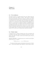
Figure 25.5.1: Endowment pattern along a Townsend turnpike.
The turnpike is of infinite extent in each direction, and has equidis-
tant trading posts. Each trading post has equal numbers of east-
heading and west-heading agents. At each trading post (the black
dots) each period, for each east-heading agent there is a west-
heading agent with whom he would like to borrow or lend. But
itineraries rule out the possibility of repayment.
The economy starts at time t =0,withN east-heading migrants and
N west-heading migrants physically located at each of the integers along a
“turnpike” of infinite length extending in both directions. Each of the integers
n =0, ±1, ±2, is a trading post number. Agents can trade the one good
only with agents at the trading post at which they find themselves at a given
date. An east-heading agent at an even-numbered trading post is endowed with
one unit of the consumption good, and an odd-numbered trading post has an

endowment of zero units (see Figure 25.5.1). A west-heading agent is endowed
with zero units at an even-numbered trading post and with one unit of the con-
sumption good at an odd-numbered trading post. Finally, at the end of each
period, each east-heading agent moves one trading post to the east, whereas
each west-heading agent moves one trading post to the west. The turnpike
along which the trading posts are located is of infinite length in each direction,
implying that the east-heading and west-heading agents who are paired at time
t will never meet again. This feature means that there can be no private debt
between agents moving in opposite directions. An IOU between agents moving
in opposite directions can never be collected because a potential lender never
Townsend’s “turnpike” interpretation 907
meets the potential borrower again; nor does the lender meet anyone who ever
meets the potential borrower, and so on, ad infinitum.
Let an agent who is endowed with one unit of the good t = 0 be called an
agent of type o and an agent who is endowed with zero units of the good at t =0
be called an agent of type e.Agentsoftypeh have preferences summarized
by

∞
t=0
β
t
u(c
h
t
). Finally, start the economy at time 0 by having each agent of
type e endowed with m
e
−1
= m units of unbacked currency and each agent of

type o endowed with m
o
−1
= 0 units of unbacked currency.
With the symbols thus reinterpreted, this model involves precisely the same
mathematics as that which was analyzed earlier. Agents’ spatial separation and
their movements along the turnpike have been set up to produce a physical rea-
son that a global market in private loans cannot exist. The various propositions
about the equilibria of the model and their optimality that were already proved
apply equally to the turnpike version.
3 , 4
Thus, in Townsend’s version of the
model, spatial separation is the “friction” that provides a potential social role
for a valued unbacked currency. The spatial separation of agents and their en-
dowment patterns give a setting in which private loan markets are limited by
theneedforpeoplewhotradeIOUstobelinked together, if only indirectly,
recurrently over time and space.
3
A version of the model could be constructed in which local private markets for
loans coexist with valued unbacked currency. To build such a model, one would
assume some heterogeneity in the time patterns of the endowment of agents who
are located at the same trading post and are headed in the same direction. If
half of the east-headed agents located at trading post i at time t have present
and future endowment pattern y
h
t
=(α, γ, α, γ . . .), for example, whereas the
other half of the east-headed agents have (γ,α,γ,α, )withγ = α, then there
is room for local private loans among this cohort of east-headed agents. Whether
or not there exists an equilibrium with valued currency depends on how nearly

Pareto optimal the equilibrium with local loan markets is.
4
Narayana Kocherlakota (1998) has analyzed the frictions in the Townsend
turnpike and overlapping generations model. By permitting agents to use history-
dependent decision rules, he has been able to support optimal allocations with
the equilibrium of a gift-giving game. Those equilibria leave no room for valued
fiat currency. Thus, Kocherlakota’s view is that the frictions that give valued
currency in the Townsend turnpike must include the restrictions on the strategy
space that Townsend implicitly imposed.
908 Credit and Currency
25.6. The Friedman rule
Friedman’s proposal to pay interest on currency by engineering a deflation can
be used to solve for a Pareto optimal allocation in this economy. Friedman’s
proposal is to decrease the currency stock by means of lump-sum taxes at a
properly chosen rate. Let the government’s budget constraint be
M
t
=(1+τ)M
t−1
.
There are N households of each type. At time t, the government transfers or
taxes nominal balances in amount τM
t−1
/(2N ) to each household of each type.
The total transfer at time t is thus τM
t−1
, because there are 2N households
receiving transfers.
The household’s time-t budget constraint becomes
p

t
c
t
+ m
t
≤ p
t
y
t
+
τ
2
M
t−1
N
+ m
t−1
.
We guess an equilibrium allocation of the same periodic pattern (25.4.3).
For the price level, we make the “quantity theory” guess M
t
/p
t
= k ,wherek
is a constant. Substituting this guess into the government’s budget constraint
gives
M
t
p
t

=(1+τ)
M
t−1
p
t−1
p
t−1
p
t
or
k =(1+τ)k
p
t−1
p
t
,
or
p
t
=(1+τ)p
t−1
, (25.6.1)
which is our guess for the price level.
Substituting the price level guess and the allocation guess into the odd agent’s
first-order condition (25.4.2) at t = 0 and rearranging shows that c
0
is now the
root of
1
(1 + τ)

−
u

(c
0
)
βu

(1 − c
0
)
=0. (25.6.2)
The price level at time t = 0 can be determined by evaluating the odd agent’s
time-0 budget constraint at m
o
−1
=0 and m
o
0
= M
0
/N =(1+τ)M
−1
/N ,with
the result that
(1 − c
0
)p
0
=

M
−1
N

1+
τ
2

.
The Friedman rule 909
Finally, the allocation guess must also satisfy the even agent’s first-order
condition (25.4.2) at t = 0 but not necessarily with equality since the stationary
equilibrium has m
e
0
= 0. After substituting (c
e
0
,c
e
1
)=(1−c
0
,c
0
)and(25.6.1)
into (25.4.2), we have
1
1+τ
≤

u

(1 − c
0
)
βu

(c
0
)
. (25.6.3)
The substitution of (25.6.2) into (25.6.3 ) yields a restriction on the set of peri-
odic allocations of type (25.4.3) that can be supported as one of our stationary
monetary equilibria,

u

(c
0
)
u

(1 − c
0
)

2
≤ 1=⇒ c
0
≥ 0.5.

This restriction on c
0
, together with (25.6.2), implies a corresponding restriction
on the set of permissible monetary/fiscal policies, 1 + τ ≥ β .
25.6.1. Welfare
For allocations of the class (25.4.3), the utility functionals of odd and even
agents, respectively, take values that are functions of the single parameter c
0
,
namely,
U
o
(c
0
)=
u(c
0
)+βu(1 −c
0
)
1 −β
2
,
U
e
(c
0
)=
u(1 − c
0

)+βu(c
0
)
1 −β
2
.
Both expressions are strictly concave in c
0
, with derivatives
U
o

(c
0
)=
u

(c
0
) − βu

(1 − c
0
)
1 −β
2
,
U
e


(c
0
)=
−u

(1 − c
0
)+βu

(c
0
)
1 −β
2
.
The Inada condition (25.2.1) ensures strictly interior maxima with respect to
c
0
. For the odd agents, the preferred c
0
satisfies U
o

(c
0
)=0,or
u

(c
0

)
βu

(1 − c
0
)
=1, (25.6.4)
910 Credit and Currency
which by (25.6.2) is the zero-inflation equilibrium, τ = 0. For the even agents,
the preferred allocation given by U
e

(c
0
) = 0 implies c
0
< 0.5, and can there-
fore not be implemented as a monetary equilibrium above. Hence, the even
agents’ preferred stationary monetary equilibrium is the one with the smallest
permissible c
0
, i.e., c
0
=0.5. According to (25.6.2), this allocation can be
supported by choosing money growth rate 1 + τ = β whichisthenalsothe
equilibrium gross rate of deflation. Notice that all agents, both odd and even,
are in agreement that they prefer no inflation to positive inflation, that is, they
prefer c
0
determined by (25.6.4) to any higher value of c

0
.
To abstract from the described conflict of interest between odd and even
agents, suppose that the agents must pick their preferred monetary policy under
a “veil of ignorance,” before knowing their true identity. Since there are equal
numbers of each type of agent, an individual faces a fifty-fifty chance of her
identity being an odd or an even agent. Hence, prior to knowing one’s identity,
the expected lifetime utility of an agent is
¯
U(c
0
) ≡
1
2
U
o
(c
0
)+
1
2
U
e
(c
0
)=
u(c
0
)+u(1 − c
0

)
2(1 − β)
.
The ex ante preferred allocation c
0
is determined by the first-order condition
¯
U

(c
0
) = 0, which has the solution c
0
=0.5. Collecting equations (25.6.1),
(25.6.2) and (25.6.3), this preferred policy is characterized by
p
t
p
t+1
=
1
1+τ
=
u

(c
o
t
)
βu


(c
o
t+1
)
=
u

(c
e
t
)
βu

(c
e
t+1
)
=
1
β
, ∀t ≥ 0,
where c
i
j
=0.5 for all j ≥ 0andi ∈{o, e}. Thus, the real return on money,
p
t
/p
t+1

, equals a common marginal rate of intertemporal substitution, β
−1
,
and this return would therefore also constitute the real interest rate if there
were a credit market. Moreover, since the gross real return on money is the
inverse of the gross inflation rate, it follows that the gross real interest rate β
−1
multiplied by the gross rate of inflation is unity, or the net nominal interest rate
is zero. In other words, all agents are ex ante in favor of Friedman’s rule.
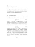
Figure 25.6.1 shows the “utility possibility frontier” associated with this econ-
omy. Except for the allocation associated with Friedman’s rule, the allocations
associated with stationary monetary equilibria lie inside the utility possibility
frontier.
Inflationary finance 911
o
U
e
U
Friedman’s Rule
Arrow Debreu
Zero Inflation Monetary
Equilibrium
A
B
C
Figure 25.6.1: Utility possibility frontier in Townsend turnpike.
The locus of points ABC denotes allocations attainable in station-
ary monetary equilibria. The point B is the allocation associated
with the zero-inflation monetary equilibrium. Point A is associated
with Friedman’s rule, while points between B and C correspond

to stationary monetary equilibria with inflation.
25.7. Inflationary finance
The government prints new currency in total amount M
t
−M
t−1
in period t and
uses it to purchase a constant amount G of goods in period t.Thegovernment’s
time-t budget constraint is
M
t
− M
t−1
= p
t
G, t ≥ 0. (25.7.1)
912 Credit and Currency
Preferences and endowment patterns of odd and even agents are as specified
previously. We now use the following definition:
Definition 4: A competitive equilibrium is a price level sequence {p
t
}
∞
t=0
,a
money supply process {M
t
}
∞
t=−1

, an allocation {c
o
t
,c
e
t
,G
t
}
∞
t=0
and nonnegative
money holdings {m
o
t
,m
e
t
}
∞
t=−1
such that
(1) Given the price sequence and (m
o
−1
,m
e
−1
), the allocation solves the optimum
problems of households of both types.

(2) The government’s budget constraint is satisfied for all t ≥ 0.
(3) N(c
o
t
+ c
e
t
)+G
t
= N , for all t ≥ 0; and m
o
t
+ m
e
t
= M
t
/N , for all t ≥−1.
For t ≥ 1, write the government’s budget constraint as
M
t
Np
t
=
p
t−1
p
t
M
t−1

Np
t−1
+
G
N
,
or
˜m
t
= R
t−1
˜m
t−1
+ g, (25.7.2)
where g = G/N ,˜m
t
= M
t
/(Np
t
) is per-odd-person real balances, and R
t−1
=
p
t−1
/p
t
is the rate of return on currency from t −1tot.
To compute an equilibrium, we guess an allocation of the periodic form
{c

o
t
}
∞
t=0
= {c
0
, 1 −c
0
− g,c
0
, 1 −c
0
− g, },
{c
e
t
}
∞
t=0
= {1 − c
0
− g,c
0
, 1 −c
0
− g,c
0
, }.
(25.7.3)

We guess that R
t
= R for all t ≥ 0, and again guess a “quantity theory”
outcome
˜m
t
=˜m ∀t ≥ 0.
Evaluating the odd household’s time-0 first-order condition for currency at
equality gives
βR =
u

(c
0
)
u

(1 − c
0
− g)
. (25.7.4)
With our guess, real balances held by each odd agent at the end of period 0,
m
o
0
/p
0
,equal1−c
0
, and time-1 consumption, which also is R times the value of

these real balances held from 0 to 1, is 1−c
0
−g.Thus,(1−c
0
)R =(1−c
0
−g),
or
R =
1 −c
0
− g
1 −c
0
. (25.7.5)
Inflationary finance 913
Equations (25.7.4) and (25.7.5) are two simultaneous equations that we want
to solve for (c
0
,R).
Use equation (25.7.5) to eliminate (1 −c
0
−g) from equation (25.7.4) to get
βR =
u

(c
0
)
u


[R(1 − c
0
)]
.
Recalling that (1 − c
0
)=m
0
, this can be written
βR =
u

(1 − m
0
)
u

(Rm
0
)
. (25.7.6)
For the power utility function u(c)=
c
1−δ
1−δ
, this equation can be solved for m
0
to get the demand function for currency
m

0
=˜m(R) ≡
(βR
1−δ
)
1/δ
1+(βR
1−δ
)
1/δ
. (25.7.7)
Substituting this into the government budget constraint (25.7.2) gives
˜m(R)(1 − R)=g. (25.7.8)
This equation equates the revenue from the inflation tax, namely, ˜m(R)(1 −R)
to the government deficit, g . The revenue from the inflation tax is the product
of real balances and the inflation tax rate 1 − R. The equilibrium value of R
solves equation (25.7.8).
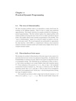
Figures 25.7.1 and 25.7.2 depict the determination of the stationary equilib-
rium value of R for two sets of parameter values. For the case δ =2,shown
in Figure 25.7.1, there is a unique equilibrium R; there is a unique equilibrium
for every δ ≥ 1. For δ ≥ 1, the demand function for currency slopes upward
as a function of R, as for the example in Figure 25.7.3. 18.6. For δ<1, there
can occur multiple stationary equilibria, as for the example in Figure 25.7.2.In
such cases, there is a Laffer curve in the revenue from the inflation tax. Notice
that the demand for real balances is downward sloping as a function of R when
δ<1.
The initial price level is determined by the time-0 budget constraint of the
government, evaluated at equilibrium time-0 real balances. In particular, the
time-0 government budget constraint can be written
M

0
Np
0
−
M
−1
Np
0
= g,
914 Credit and Currency
0
0.1
0.2
0.3
0.4
0.5
0.6
0.7
0.8
0.9
0
0.1 0.2 0.3 0.4 0.5 0.6 0.7 0.8 0.9 1
Figure 25.7.1: Revenue from inflation tax
[m(R)(1−R)] and deficit for β = .95,δ=2,g = .2. The gross rate
of return on currency is on the x-axis; the revenue from inflation
and g are on the y -axis.
0
0.05
0.1
0.15

0.2
0.25
0.3
0
0.1 0.2 0.3 0.4 0.5 0.6 0.7 0.8 0.9 1
Figure 25.7.2: Revenue from inflation tax
[m(R)(1 −R)] and deficit for β = .95,δ = .7,g = .2. Therateof
return on currency is on the x-axis; the revenue from inflation and
g are on the y -axis. Here there is a Laffer curve.
Inflationary finance 915
0.1
0.15
0.2
0.25
0.3
0.35
0.4
0.45
0.5
0
0.1 0.2 0.3 0.4 0.5 0.6 0.7 0.8 0.9 1
Figure 25.7.3: Demand for real balances on the y-axisasfunction
of the gross rate of return on currency on x-axis when β = .95,δ=
2.
0.45
0.5
0.55
0.6
0.65
0.7

0.75
0.8
0.85
0.9
0.95
0
0.1 0.2 0.3 0.4 0.5 0.6 0.7 0.8 0.9 1
Figure 25.7.4: Demand for real balances on the y-axisasfunction
of the gross rate of return on currency on x-axis when β = .95,δ=
.7.
916 Credit and Currency
or
˜m − g =
M
−1
Np
0
.
Equating ˜m to its equilibrium value 1 −c
0
and solving for p
0
gives
p
0
=
M
−1
N(1 − c
0

− g)
.
25.8. Legal restrictions
This section adapts ideas of Bryant and Wallace (1984) to the turnpike environ-
ment. Bryant and Wallace and Villamil (1988) analyzed situations in which the
government could make all savers better off by introducing a price discrimination
scheme for marketing its debt. The analysis formalizes some ideas mentioned
by John Maynard Keynes (1940).
Figure 25.8.1 depicts the terms on which an odd agent at t =0 cantransfer
consumption between 0 and 1 in an equilibrium with inflationary finance. The
agent is endowed at the point (1, 0). The monetary mechanism allows him to
transfer consumption between periods on the terms c
1
= R(1 −c
0
), depicted by
the budget line connecting 1 on the c
t
-axis with the point B on the c
t+1
-axis.
The government insists on raising revenues in the amount g for each pair of an
odd and an even agent, which means that R must be set so that the tangency
between the agent’s indifference curve and the budget line c
1
= R(1−c
0
) occurs
at the intersection of the budget line and the straight line connecting 1 − g on
the c

t
-axis with the point 1 − g on the c
t+1
-axis. At this point, the marginal
rate of substitution for odd agents is
u

(c
0
)
βu

(1 − c
0
− g)
= R,
(because currency holdings are positive). For even agents, the marginal rate of
substitution is
u

(1 − c
0
− g)
βu

(c
0
)
=
1

β
2
R
> 1,
where the inequality follows from the fact that R<1 under inflationary finance.
Legal restrictions 917
c
t+1
c
t
1-g
1-g
1
1
c = R(1-c )
0
1
I
A
B
1-F
H
D
Figure 25.8.1: The budget line starting at (1, 0) and ending
at the point B describes an odd agent’s time-0 opportunities in
an equilibrium with inflationary finance. Because this equilibrium
has the “private consumption feasibility menu” intersecting the
odd agent’s indifference curve, a “forced saving” legal restriction
can be used to put the odd agent onto a higher indifference curve
than I, while leaving even agents better off and the government

with revenue g . If the individual is confronted with a minimum
denomination F at the rate of return associated with the budget
line ending at H, he would choose to consume 1 −F .
The fact that the odd agent’s indifference curve intersects the solid line con-
necting (1 − g) on the two axes indicates that the government could improve
the welfare of the odd agent by offering him a higher rate of return subject to a
minimal real balance constraint. The higher rate of return is used to send the
line c
1
=(1−R)c
0
into the “lens-shaped area” in Figure 25.8.1 onto a higher
918 Credit and Currency
indifference curve. The minimal real balance constraint is designed to force the
agent onto the “post–government share” feasibility line connecting the points
1 −g on the two axes.
Thus, notice that in Figure 25.8.1, the government can raise the same rev-
enue by offering odd agents the higher rate of return associated with the line
connecting 1 on the c
t
axis with the point H on the c
t+1
axis, provided that
the agent is required to save at least F , if he saves at all. This minimum saving
requirement would make the household’s budget set the point (1, 0) together
with the heavy segment DH. With the setting of F, R associated with the line
DH in Figure 25.8.1, odd households have the same two-period utility as without
this scheme. (Points D and A lie on the same indifference curve.) However, it
is apparent that there is room to lower F and lower R a bit, and thereby move
the odd household into the lens-shaped area. See Figure 25.8.2.

The marginal rates of substitution that we computed earlier indicate that
this scheme makes both odd and even agents better off relative to the original
equilibrium. The odd agents are better off because they move into the lens-
shaped area in Figure 18.8. The even agents are better off because relative
to the original equilibrium, they are being permitted to “borrow” at a gross
rate of interest of one. Since their marginal rate of substitution at the original
equilibrium is 1/(β
2
R) > 1, this ability to borrow makes them better off.
25.9. A two-money model
There are two types of currency being issued, in amounts M
it
,i =1, 2byeach
of two countries. The currencies are issued according to the rules
M
it
− M
it−1
= p
it
G
it
,i=1, 2(25.9.1)
where G
it
is total purchases of time-t goods by the government issuing currency
i,andp
it
is the time-t price level denominated in units of currency i.We
assume that currencies of both types are initially equally distributed among the

even agents at time 0. Odd agents start out with no currency.
A two-money model 919
c
t+1
c
t
1-g
1-g
1
1
c = R(1-c )
0
1
I
A
B
1-F'
H'
D
I'
E
Figure 25.8.2: The minimum denomination F and the return
on money can be lowered vis-`a-vis their setting associated with
line DH in Figure 18.8 to make the odd household better off, raise
the same revenues for the government, and leave even households
better off (as compared to no government intervention). The lower
value of F puts the odd household at E, which leaves him at
the higher indifference curve I

. The minimum denomination F

and the return on money can be lowered vis-`a-vis their setting
associated with line DH in Figure 18.8 to make the odd house-
hold better off, raise the same revenues for the government, and
leave even households better off (as compared to no government
intervention). The lower value of F puts the odd household at E ,
which leaves him at the higher indifference curve I

.
920 Credit and Currency
Household h’s optimum problem becomes to maximize

∞
t=0
β
t
u(c
h
t
) subject
to the sequence of budget constraints
c
h
t
+
m
h
1t
p
1t
+

m
h
2t
p
2t
≤ y
h
t
+
m
h
1t−1
p
1t
+
m
h
2t−1
p
2t
,
where m
h
jt−1
are nominal holdings of country j ’scurrencybyhouseholdh.
Currency holdings of each type must be nonnegative. The first-order conditions
for the household’s problem with respect to m
h
jt
for j =1, 2are

βu

(c
h
t+1
)
p
1t+1
≤
u

(c
h
t
)
p
1t
, =ifm
h
1t
> 0,
βu

(c
h
t+1
)
p
2t+1
≤

u

(c
h
t
)
p
2t
, =ifm
h
2t
> 0.
If agent h chooses to hold both currencies from t to t + 1, these first-order
conditions imply that
p
2t
p
1t
=
p
2t+1
p
1t+1
,
or
p
1t
= ep
2t
, ∀t ≥ 0, (25.9.2)

for some constant e>0.
5
This equation states that if in each period there is
some household that chooses to hold positive amounts of both types of currency,
the rate of return from t to t + 1 must be equal for the two types of currencies,
meaning that the exchange rate must be constant over time.
6
We use the following definition:
Definition 5: A competitive equilibrium with two valued fiat currencies is an
allocation {c
o
t
,c
e
t
,G
1t
,G
2t
}
∞
t=0
, nonnegative money holdings {m
o
1t
,m
e
1t
,m
o

2t
,m
e
2t
}
∞
t=−1
,
a pair of finite price level sequences {p
1t
,p
2t
}
∞
t=0
and currency supply sequences
{M
1t
,M
2t
}
∞
t=−1
such that
(1) Given the price level sequences and (m
o
1,−1
,m
e
1,−1

,m
o
2,−1
,m
e
2,−1
), the allo-
cation solves the households’ problems.
5
Evaluate both of the first-order conditions at equality, then divide one by
the other to obtain this result.
6
As long as we restrict ourselves to nonstochastic equilibria.
A two-money model 921
(2) The budget constraints of the governments are satisfied for all t ≥ 0.
(3) N(c
o
t
+ c
e
t
)+G
1t
+ G
2t
= N , for all t ≥ 0; and m
o
jt
+ m
e

jt
= M
jt
/N ,for
j =1, 2andallt ≥−1.
In the case of constant government expenditures (G
1t
,G
2t
)=(Ng
1
,Ng
2
)
for all t ≥ 0, we guess an equilibrium allocation of the form (25.7.3), where we
reinterpret g to be g = g
1
+ g
2
. We also guess an equilibrium with a constant
real value of the “world money supply,” that is,
˜m =
M
1t
Np
1t
+
M
2t
Np

2t
,
and a constant exchange rate, so that we impose condition (25.9.2). We let
R = p
1t
/p
1t+1
= p
2t
/p
2t+1
be the constant common value of the rate of return
on the two currencies.
With these guesses, the sum of the two countries’ budget constraints for
t ≥ 1 and the conjectured form of the equilibrium allocation imply an equation
of the form (25.7.8), where now
˜m(R)=
M
1t
p
1t
N
+
M
2t
p
2t
N
.
Equation (25.7.8) can be solved for R in the fashion described earlier. Once

R has been determined, so has the constant real value of the world currency
supply, ˜m. To determine the time-t price levels, we add the time-0 budget
constraints of the two governments to get
M
10
Np
10
+
M
20
Np
20
=
M
1,−1
+ eM
2,−1
Np
10
+(g
1
+ g
2
),
or
˜m −g =
M
1,−1
+ eM
2,−1

Np
10
.
In the conjectured allocation, ˜m =(1−c
0
), so this equation becomes
M
1,−1
+ eM
2,−1
Np
10
=1−c
0
− g, (25.9.3)
which, given any e>0, has a positive solution for the initial country-1 price
level. Given the solution p
10
and any e ∈ (0, ∞), the price level sequences for
the two countries are determined by the constant rate of return on currency R.