Accounting for Managers Part 5 ppt
Bạn đang xem bản rút gọn của tài liệu. Xem và tải ngay bản đầy đủ của tài liệu tại đây (193.22 KB, 33 trang )
9
Operating Decisions
This chapter introduces the operations function through the value chain and
contrasts the different operating decisions faced by manufacturing and service
businesses. Operational decisions are considered, in particular capacity utiliza-
tion, the cost of spare capacity and the product/service mix under capacity
constraints. Relevant costs are considered in relation to the make versus buy
decision, equipment replacement and the relevant cost of materials. Other costing
approaches such as lifecycle, target and kaizen costing and the cost of quality are
also introduced.
The operations function
Operations is the function that produces the goods or services to satisfy demand
from customers. This function, interpreted broadly, includes all aspects of pur-
chasing, manufacturing, distribution and logistics, whatever those may be called
in particular industries. While purchasing and logistics may be common to all
industries, manufacturing will only be relevant to a manufacturing business. There
will also be different emphases such as distribution for a retail business and the
separation of ‘front office’ (or customer-facing) functions from ‘back office’ (or
support) functions for a financial institution.
Irrespective of whether the business is in manufacturing, retailing or services,
we can consider operations as the all-encompassing processes that produce the
goods or services that satisfy customer demand. In simple terms, operations is
concerned with the conversion process between resources (materials, facilities
and equipment, people etc.) and the products/services that are sold to customers.
There are four aspects of the operations function: quality, speed, dependability and
flexibility (Slack et al., 1995). Each of these has cost implications and the lower the
cost of producing goods and services, the lower can be the price to the customer.
Lower prices tend to increase volume, leading to economies of scale such that
profits should increase (as we saw in Chapter 8).
A useful analytical tool for understanding the conversion process is the value
chain developed by Porter (1985) and shown in Figure 9.1. According to Porter
every business is:
a collection of activities that are performed to design, produce, market,
deliver, and support its product A firm’s value chain and the way it
122 ACCOUNTING FOR MANAGERS
Firm Infrastructure
Human Resource Management
Technology Development
Procurement
Inbound
Logistics
Operations Outbound
Logistics
Marketing
and Sales
Service
Support
activities
Margin
Primary
activities
Figure 9.1 Porter’s value chain
Reprinted from Porter, M. E. (1985). Competitive Advantage: Creating and Sustaining Superior Performance.
New York, NY: Free Press.
performs individual activities are a reflection of its history, its strategy, its
approach to implementing its strategy, and the underlying economics of the
activities themselves. (Porter, 1985, p. 36)
Porter separated these activities into primary and secondary activities.
This approach has similarities to the business process re-engineering approach
of Hammer and Champy (1993, p. 32). Their emphasis on processes was on ‘a
collection of activities that takes one or more kinds of input and creates an output
that is of value to the customer’ (p. 35).
Porter argued that costs should be assigned to the value chain but that account-
ing systems can get in the way of analysing those costs. Accounting systems
categorize costs through line items (see Chapter 3) such as salaries and wages,
rental, electricity etc. rather than in terms of value activities that are technologi-
cally and strategically distinct. This ‘may obscure the underlying activities a firm
performs’ (Porter, 1985).
Porter developed the notion of cost drivers, which he defined as the structural
factors that influence the cost of an activity and are ‘more or less’ under the
control of the business. He proposed that the cost drivers of each value activity be
analysed to enable comparisons with competitor value chains. This would result
in the relative cost position of the business being improved by better control of the
cost drivers or by reconfiguring the value chain, while maintaining a differentiated
product. This isan approach that is supported by strategicmanagement accounting
(see Chapter 4).
The value chain as a collection of inter-related business processes is a useful
concept to understand businesses that produce either goods or services.
Managing operations – manufacturing
A distinguishing feature between the sale of goods and services is the need for
inventory or stock in the sale of goods. Inventory enables the timing difference
OPERATING DECISIONS 123
between production capacity and customer demand to be smoothed. This is of
course not possible in the supply of services.
Manufacturing firms purchase raw materials (unprocessed goods) and under-
take the conversion process through the application of labour, machinery and
know-how to manufacture finished goods. The finished goods are then available
to be sold to customers. There are actually three types of inventory in this example:
raw materials, finished goods and work-in-progress. Work-in-progress consists
of goods that have begun but have not yet completed the conversion process.
There are different types of manufacturing and it is important to differentiate
the production of the following:
ž
Custom: Unique, custom products produced singly, e.g. a building.
ž
Batch: A quantity of the same goods produced at the same time (often called a
production run), e.g. textbooks.
ž
Continuous: Products produced in a continuous production process, e.g. oil
and chemicals.
For custom and batch manufacture, costs are collected through a job costing
system that accumulates the cost of raw materials as they are issued to each
job (either a custom product or a batch of products) and the cost of time spent
by different categories of labour. In a manufacturing business the materials are
identified by a bill of materials, a list of all the components that go to make up the
completed project, and a routing, a list of the labour or machine processing steps
and times for the conversion process. To each of these costs overhead is allocated
to cover the manufacturing costs that are not included in either the bill of materials
or the routing (this will be explained in Chapter 11).
The bill of materials and routing contain standard quantities of material and
time. Standard quantities are the expected quantities, based on past and cur-
rent experience and planned improvements in product design, purchasing and
methods of production. Standard costs are the standard quantities multiplied by
the current and anticipated purchase prices for materials and the labour rates of
pay. The standard cost is therefore a budget cost for a product or batch. As actual
costs are not known for some time after the end of the accounting period, standard
costs are generally used for decision-making. Standard costs are usually expressed
per unit.
The manufacturing process and its relationship to accounting can be seen in
Figure 9.2. When acustom product iscompleted, the accumulated cost ofmaterials,
labour and overhead is the cost of that custom product. For a batch the total job
cost is divided by the number of units produced (e.g. the number of copies of the
textbook) to give a cost per unit (cost per textbook). The actual cost per unit can
be compared to the budget or standard cost per unit. Any variation needs to be
investigated and corrective action taken (this is the feedback cycle described in
Chapter 4, to which we return in Chapter 15).
A simple example is the job cost for the printing of 5,000 copies of a textbook.
The costing system shows:
124 ACCOUNTING FOR MANAGERS
INPUTS CONVERSION PROCESS OUTPUTS
Custom
Batch
Continuous
Raw materials Work-in-progress Finished goods
+
Labour
Equipment, facilities, space etc.
Bill of materials
Components and quantities
Labour routing
Processing steps and times
which are priced to become
Standard costs
+
Figure 9.2 The manufacturing process and its relationship to accounting
Materials (paper, ink etc.) £12,000
Labour for printing £20,000
Overhead allocated £10,000
Total job cost £42,000
Cost per textbook (£42,000/5,000 copies) £8.40
For continuous manufacture a process costing system is used, under which costs
are collected over a period of time, together with a measure of the volume of
production. At the end of the accounting period, the total costs are divided
by the volume produced to give a cost per unit of volume. For example, if
the cost of producing a chemical in the month of November is £1,200,000 and
400,000 litres have been produced in the same period, the cost per litre is £3.00
(£1,200,000/400,000 litres). Again, there will be a comparison between the standard
cost per unit and the actual cost per unit.
The distinction between custom and batch is not always clear. Some products
are produced on an assembly line as a batch of similar units but with some
customization, since technology allows each unit to be unique. For example, motor
vehicles are assembled as ‘batches of one’, since technology facilitates the sequenc-
ing of different specifications for each vehicle along a common production line.
Within the same model, different colours, transmissions (manual or automatic),
steering (right-hand or left-hand drive) etc. can all be accommodated.
Any manufacturing operation involves a number of sequential activities that
need to be scheduled so that materials arrive at the appropriate time at the correct
OPERATING DECISIONS 125
stage of production and labour is available to carry out the required process.
Organizations that aim to have material arrive in production without holding
buffer stocks are said to operate a just-in-time (or JIT) manufacturing system.
Most manufacturing processes require an element of set-up or make-ready time,
during which equipment settings are made to meet the specifications of the next
production run (a custom product or batch). These settings may be made by
manual labour or by computer through CNC (computer numerical control) tech-
nology. As Chapter 1 described, investments in computer and robotics technology
have changed the shape of manufacturing industry. These investments involve
substantial costs that need to be justified by an increased volume of production or
by efficiencies that reduce production costs (we discuss this in Chapter 12).
Managing operations – services
Fitzgerald et al. (1991) emphasized the importance of the growing service sector
and identified four key differences between products and services: intangibility,
heterogeneity, simultaneity and perishability. Services are intangible rather than
physical and are often delivered in a ‘bundle’ such that customers may value
different aspects of the service. Services involving high labour content are hetero-
geneous, i.e. the consistency of the service may vary significantly. The production
and consumption of services are simultaneous so that services cannot be inspected
before they are delivered. Services are also perishable, so that unlike physical goods,
there can be no stock of services that have been provided but remain unsold.
Fitzgerald et al. also identified three different service types. Professional services
are ‘front office’, people based, involving discretion and the customization of
services to meet customer needs in which the process is more important than the
service itself. Examples given by Fitzgerald et al. include professional firms such
as solicitors, auditors and management consultants. Mass services involve limited
contact time by staff and little customization, with services equipment based
and product oriented with an emphasis on the ‘back office’ and little autonomy.
Examples here are rail transport, airports and mass retailing. The third type of
service is the service shop, a mixture of the other two extremes with emphasis on
front and back office, people and equipment and product and process. Examples
of service shops are banking and hotels.
Fitzgerald et al. emphasized how cost traceability differed between each of
these service types. Their research found that many service companies did not
try to cost individual services accurately either for price-setting or profitability
analysis, except for the time-recording practices of professional service firms. In
mass services and service shops there were:
multiple, heterogeneous and joint, inseparable services, compounded by the
fact that individual customers may consume different mixes of services and
may take different routes through the service process. (p. 24)
In these two categories of services, costs were controlled not by collecting the costs
of each service but through responsibility centres (which is covered in more detail
in Chapter 13).
126 ACCOUNTING FOR MANAGERS
Slack et al. (1995) contrasted types of service provision with types of manu-
facturing and used a matrix of low volume/high variety and high volume/low
variety to compare professional service with customized or batch manufacturing,
mass service with continuous manufacture, and service shop with a batch-type
process. Slack et al. noted that this product–process matrix led to decisions about
the design of the operations function, while deviating from these broad groups
had implications for both flexibility and cost.
In describing operations, we will use the term production to refer to both
goods and services and use manufacturing where raw materials are converted into
finished goods.
Accounting information has an important part to play in operational decisions.
Typical questions that may arise include:
ž
What is the cost of spare capacity?
ž
What product/service mix should be produced where there are capacity con-
straints?
ž
What are the costs that are relevant for operational decisions?
Accounting for the cost of spare capacity
Production resources (material, facilities and equipment, and people) allocated to
the process of supplying goods and services provide a capacity. The utilization
of that capacity is a crucial performance driver for businesses, as the investment
in capacity often involves substantial outlays of funds that need to be recovered
by utilizing that capacity fully in the production of products/services. Capacity
may also be a limitation for the production and distribution of goods and services
where market demand exceeds capacity.
A weakness of traditional accounting is that it equates the cost of using resources
with the cost of supplying resources. Activity-based costing (which is described
further in Chapters 10 and 11) has as a central focus the identification and
elimination of unused capacity. According to Kaplan and Cooper (1998), there are
two ways in which unused capacity can be eliminated:
1 Reducing the supply of resources that perform an activity, i.e. spending reduc-
tions that reduce capacity.
2 Increasing the quantity of activities for the resources, i.e. revenue increases
through greater utilization of existing capacity.
Activity-based costing identifies the difference between the cost of resources
supplied and the cost of resources used as the cost of the unused capacity:
cost of resources supplied − cost of resources used = cost of unused capacity
An example illustrates this.
Ten staff, each costing £30,000 per year, deliver banking services where the
cost driver (the cause of the activity) is the number of banking transactions.
OPERATING DECISIONS 127
Assuming that each member of staff can process 2,000 transactions per annum,
the cost of resources supplied is £300,000 (10 × £30,000) and the capacity number
of transactions is 20,000 (10 × 2,000). The standard cost per transaction would be
£15 (£300,000/20,000 transactions).
If in fact 18,000 transactions were carried out in the year, the cost of resources
used would be £270,000 (18,000 @ £15) and the cost of unused capacity would be
£30,000 (2,000 @ £15, or £300,000 resources supplied − £270,000 resources used).
If the cost of resources used is equated with the cost of resources supplied,
the actual transaction cost becomes £16.67 (£300,000/18,000 transactions) and
the cost of unused capacity is not identified. This is a weakness of traditional
accounting systems.
Although there can be no carry forward of an ‘inventory’ of unused capacity
in a service delivery function, management information is more meaningful if
the standard cost is maintained at £15 and the cost of spare capacity is identified
separately. Management action can then be taken to reduce the cost of spare
capacity to zero, either by increasing the volume of business or reducing the
capacity (i.e. the number of staff).
Capacity utilization and product mix
Where demand exceeds the capacity of the business to produce goods or deliver
services as a result of scarce resources (whether that is space, equipment, materials
or staff), the scarce resource is the limiting factor. A business will want to
maximize its profitability by selecting the optimum product/service mix. The
product/service mix is the mix of products or services sold by the business, each
of which may have different selling prices and costs. It is therefore necessary,
where demand exceeds capacity, to rank the products/services with the highest
contributions, per unit of the limiting factor (i.e. the scarce resource).
For example, Beaufort Accessories makes three parts (F, G and H) for a motor
vehicle, each with different selling prices and variable costs and requiring a
different number of machining hours. These are shown in Table 9.1. However,
Beaufort has an overall capacity limitation of 10,000 machine hours.
Table 9.1 Beaufort accessories cost information
Part F Part G Part H
Selling price per unit £150 £200 £225
Variable material cost per unit £50 £80 £40
Variable labour cost per unit £50 £60 £125
Contribution per unit £50 £60 £60
Machine hours per unit 2 4 5
Estimated sales demand (units) 2,000 2,000 2,000
Required machine hours based
on estimated demand
4,000 8,000 10,000
128 ACCOUNTING FOR MANAGERS
Table 9.2 Beaufort accessories – product ranking based on
contribution
Part F Part G Part H
Contribution per unit £50 £60 £60
Machine hours per unit 2 4 5
Contribution per machine hour £25 £15 £12
Ranking (preference) 1 2 3
The first step is to identify the ranking of the products by calculating the
contribution per unit of the limiting factor (machine hours in this case) for each
product. This is shown in Table 9.2.
Although both Part G and Part H have higher contributions per unit, the
contribution per machine hour (the unit of limited capacity) is higher for Part F.
Profitability will be maximized by using the limited capacity to produce as many
Part Fs as can be sold, followed by Part Gs. Based on this ranking, the available
production capacity can be allocated as follows:
Production Contribution
2,000 of Part F @ 2 hours = 4,000 hours. 2,000 @ £50 per unit = £100,000
Based on the capacity limitation of
10,000 hours, there are 6,000 hours
remaining, so Beaufort can produce 3/4
of the demand for Part G (6,000 hours
available/8,000 hours to meet demand)
equivalent to 1,500 units of part G (3/4
of 2,000 units).
1,500 of Part G @ 4 hours = 6,000 hours 1,500 @ £60 per unit = £90,000
Maximum contribution £190,000
There is no available capacity for Part H.
Theory of Constraints
A different approach to limited capacity was developed by Goldratt and Cox
(1986), who focused on the existence of bottlenecks in production and the need
to maximize volume through the bottleneck (throughput). Goldratt and Cox
developed the Theory of Constraints (ToC), under which only three aspects
of performance are important: throughput contribution, operating expense and
inventory. Throughput contribution is defined as sales revenue less the cost
of materials:
throughput contribution = sales − cost of materials
OPERATING DECISIONS 129
Table 9.3 Beaufort accessories – product ranking based on throughput
Part F Part G Part H
Selling price per unit £150 £200 £225
Variable material cost per unit £50 £80 £40
Throughput contribution per unit £100 £120 £185
Machine hours per unit 2 4 5
Return per machine hour £50 £30 £37
Ranking (preference) 1 3 2
Goldratt and Cox considered all other costs as fixed and independent of customers
and products, so operating expenses included all costs except materials. They
emphasized the importance of maximizing throughput while holding constant
or reducing operating expenses and inventory. Goldratt and Cox also recognized
that there is little point in maximizing non-bottleneck resources if this leads to an
inability to produce at the bottlenecks.
Applying the Theory of Constraints to the Beaufort Accessories example and
assuming that machine hours are the bottleneck resource, Table 9.3 shows the
throughput ranking. Under the Theory of Constraints, Part F retains the highest
ranking but Part H has a higher return per unit of the bottleneck resource than Part
G after deducting only the variable cost of materials. This is a different ranking
to the previous method, which used the contribution after deducting all variable
costs. The difference is due to the treatment of variable costs other than materials.
Strategic management accounting (see Chapter 4) can assist a business by
applying these concepts to competitors in order to gain a better understanding
of how those competitors are utilizing their capacity. Understanding their irrel-
ative strengths and weaknesses can result in gaining competitive advantage in
the market.
Operating decisions: relevant costs
Operating decisions imply an understanding of costs, but not necessarily those
costs that are defined by accountants. We have already seen in Chapter 8 the
distinction between avoidable and unavoidable costs. This brings us to the notion
of relevant costs. Relevant costs are those costs that are relevant to a particular
decision. Relevant costs are the future, incremental cash flows that result from a
decision. Relevant costs specifically do not include sunk costs, i.e. costs that have
been incurred in the past, as nothing we can do can change those earlier decisions.
Relevant costs are avoidable costs because, by taking a particular decision, we
can avoid the cost. Unavoidable costs are not relevant because, irrespective of
what our decision is, we will still incur the cost. Relevant costs may, however, be
opportunity costs. An opportunity cost is not a cost that is paid out in cash. It is the
loss of a future cash flow that takes place as a result of making a particular decision.
130 ACCOUNTING FOR MANAGERS
Make versus buy?
A concern with subcontracting or outsourcing has dominated business in recent
years as the cost of providing goods and services in-house is increasingly compared
to the cost of purchasing goods on the open market. The make versus buy decision
should be based on which alternative is less costly on a relevant cost basis, that is
taking into account only future, incremental cash flows.
For example, the costs of in-house production of a computer processing service
that averages 10,000 transactions per month are calculated as £25,000 per month.
This comprises £0.50 per transaction for stationery and £2 per transaction for
labour. In addition, there is a £10,000 charge from head office as the share of
the depreciation charge for equipment. An independent computer bureau has
tendered a fixed price of £20,000 per month.
Based on this information, stationery and labour costs are variable costs that are
both avoidable if processing is outsourced. The depreciation charge is likely to be
a fixed cost to the business irrespective of the outsourcing decision. It is therefore
unavoidable. The fixed outsourcing cost will only be incurred if outsourcing
takes place.
The relevant costs for each alternative can be compared as shown in Table 9.4.
The £10,000 share of depreciation costs is not relevant as it is unavoidable. The
relevant costs for this decision are therefore those shown in Table 9.5.
Based on relevant costs, there would be a £5,000 per month saving by outsourc-
ing the computer processing service.
Table 9.4 Relevant costs – make versus buy
Cost to make Cost to buy
Stationery 5,000
10,000 @ £0.50
Labour 20,000
10,000 @ £2
Share of depreciation costs 10,000 10,000
Outsourcing cost 20,000
Total relevant cost £35,000 £30,000
Table 9.5 Relevant costs – make versus buy, simplified
Relevant cost to make Relevant cost to buy
Stationery 5,000
10,000 @ £0.50
Labour 20,000
10,000 @ £2
Outsourcing cost 20,000
Total relevant cost £25,000 £20,000
OPERATING DECISIONS 131
Equipment replacement
A further example of the use of relevant costs is in the decision to replace plant
and equipment. Once again, the concern is with future incremental cash flows, not
with historical or sunk costs or with non-cash expenses such as depreciation.
Mammoth Hotel Company replaced its kitchen one year ago at a cost of
£120,000. The kitchen was to be depreciated over five years, although it will still
be operational after that time. The hotel manager wishes to expand the dining
facility and needs a larger kitchen with additional capacity. A new kitchen will
cost £150,000, but the kitchen equipment supplier is prepared to offer £25,000 as
a trade-in for the old kitchen. The new kitchen will ensure that the dining facility
earns additional income of £25,000 for each of the next five years.
The existing kitchen incurs operating costs of £40,000 per year. Due to labour
saving technology, operating costs, even with additional dining, will fall to £30,000
per year if the new kitchen is bought. These figures are shown in Table 9.6. On a
relevant cost basis, the difference between retaining the old kitchen and buying
the new kitchen is a saving of £50,000 cash flow over five years. On this basis, it
makes sense to buy the new kitchen.
The original kitchen cost has been written down to £96,000 (cost of £120,000 less
one year’s depreciation at 20% or £24,000). The original capital cost is a sunk cost
and is therefore irrelevant to a future decision. The loss on sale of £71,000 (£96,000
writtendownvalue− £25,000 trade-in) will affect the hotel’s reported profit, but
it is not a future incremental cash flow and is therefore irrelevant to the decision.
However, there is a tension between a decision based on future incremental cash
flows and the reported financial position that will show a significant (non-cash)
financial loss in the year in which the old kitchen is written off. The political
aspects of such a decision were discussed in Chapter 5. Other aspects of capital
expenditure decisions are explained in Chapter 12.
Relevant cost of materials
As the definition of relevant cost is the future incremental cash flow, it follows
that the relevant cost of direct materials is not the historical (or sunk) cost but the
Table 9.6 Relevant costs – equipment replacement
Retain old kitchen Buy new kitchen
Purchase price of new kitchen −£150,000
Trade-in value of old machine +£25,000
Operating costs
£40,000 p.a. × 5years −£200,000
£30,000 p.a. × 5years −£150,000
Additional income from dining of
£25,000 p.a. × 5years
+£125,000
Total relevant cost −£200,000 −£150,000
132 ACCOUNTING FOR MANAGERS
replacement price of the materials. Therefore it is irrelevant whether or not those
materials are held in inventory, unless such materials have only scrap value or
an alternative use, in which case the relevant cost is the opportunity cost of the
forgone alternative. The cost of using materials can be summarized as follows:
ž
If the material is purchased specifically the relevant cost is the purchase price.
ž
If the material is already in stock and is used regularly, the relevant cost is the
purchase price (i.e. the replacement price).
ž
If the material is already in stock but is surplus as a result of previous
overbuying, the relevant cost is the opportunity cost, which may be its scrap
value or its value in any alternative use.
Stanford Potteries Ltd has been approached by a customer who wants to place a
special order and is willing to pay £16,000. The order requires the materials shown
in Table 9.7.
Material A would have to be purchased specifically for this order. Material B is
used regularly and any inventory used for this order would have to be replaced.
Material C is surplus to requirements and has no alternative use. Material D
is also surplus to requirements but can be used as a substitute for material E.
Material E, although not required for this order, is in regular use and currently
costs £8.00 per kg, but is not in stock. The relevant material costs are shown in
Table 9.8.
As a result of the above, Stanford Potteries would accept the special order
because the additional income exceeds the relevant cost of materials. In the case
of A, the material is purchased at the current purchase price. For B, even though
some inventory is held at a lower cost price, it is used regularly and has to be
replaced at the current purchase price. For C, the 400 kg in inventory have no
other value than scrap, which is the opportunity cost of using it in this order. The
100 kg of C not in inventory have to be purchased at the current replacement price.
For D, the opportunity cost is either the scrap value or the saving made by using
material D as a substitute for material E. As the substitution value is higher, this
is what Stanford would do in the absence of this particular order. Therefore, the
opportunity cost of D is the loss of the ability to substitute for material E.
Relevant costs are a useful tool in helping to make operational decisions.
However, there are other approaches to costing that are also valuable.
Table 9.7 Material requirements
Material Total kg
required
Kg in stock Original
purchase price
per kg
Scrap value
per kg
Current
purchase
price per kg
A 750 0 – – 6.00
B 1,000 600 3.50 2.50 5.00
C 500 400 3.00 2.50 4.00
D 300 500 4.00 6.00 9.00
OPERATING DECISIONS 133
Table 9.8 Relevant cost of materials
Material Relevant cost
A 750 @ £6 (replacement price) 4,500
B 1,000 @ £5 (replacement price) 5,000
C 400 @ £2.50 (opportunity cost of scrap value) 1,000
100 @ £4 (replacement price) 400
D 300 @ £6 (opportunity cost of scrap value) 1,800
or
300 @ £8 (substitute for material E) 2,400
Total relevant material cost 13,300
Proceeds of sale 16,000
Incremental gain 2,700
Other costing approaches
Lifecycle costing
All products and services go through a typical lifecycle, from introduction, through
growth and maturity to decline. The lifecycle is represented in Figure 9.3.
Over time, sales volume increases, then plateaus and eventually declines.
Management accounting has traditionally focused on the period after product
design and development, when the product/service is in production for sale to
customers. However, the product design phase involves substantial costs that
may not be taken into account in product/service costing. These costs may have
been capitalized (see Chapters 3 and 6) or treated as an expense in earlier years.
Similarly, when products/services are discontinued, the costs of discontinuance
are rarely identified as part of the product/service cost.
Lifecycle costing estimates and accumulates the costs of a product/service
over its entire lifecycle, from inception to abandonment. This helps to deter-
mine whether the profits generated during the production phase cover all the
lifecycle costs. This information helps managers make decisions about future
product/service development and the need for cost control during the develop-
ment phase.
Sales
volume
Introduction Growth Maturity Decline
Figure 9.3 Typical product/service lifecycle
134 ACCOUNTING FOR MANAGERS
The design and development phase can determine up to 80% of costs in many
advanced technology industries. This is because decisions about the production
process and the technology investment required to support production are made
long before the product/servicesareactuallyproduced. This is shown in Figure 9.4.
Consequently, efforts to reduce costs during the production phase are unlikely
to be successful when the costs are committed or locked in as a result of technology
and process decisions made during the design phase.
Target costing
Target costing is concerned with managing whole-of-life costs during the design
phase. It has four stages:
1 Determining the target price that customers will be prepared to pay for the
product/service.
2 Deducting a target profit margin to determine the target cost, which becomes
the cost to which the product/service should be engineered.
3 Estimating the actual cost of the product/service based on the current design.
4 Investigating ways of reducing the estimated cost to the target cost.
target price − target profit margin = target cost
The technique was developed in the Japanese automotive industry and is customer
oriented. Its aim was to build a product at a cost that could be recovered over the
product lifecycle through a price that customers would be willing to pay to obtain
the benefits (which in turn drive the product cost).
Target costing is equally applicable to a service. The design of an Internet
banking service involves substantial up-front investment, the benefits of which
must be recoverable in the selling price over the expected lifecycle of the service.
Using a simple example, a new product is expected to achieve a desired volume
and market share at a price of £1,000, from which the manufacturer wants a 20%
margin, leaving a target cost of £800. Current estimates suggest the cost as £900. An
investigation seeks to find which elements of design, manufacture or purchasing
contribute to the costs and how those costs can be reduced, or whether features
£ Capital investment
Design phase
Launch Production phase
Figure 9.4 Investment decisions
OPERATING DECISIONS 135
can be eliminated that cannot be justified in the target price. This is an iterative
process, but an essential one if the lifecycle costs of the product/service are to be
managed and recovered in the (target) selling price. Importantly, this process of
estimating costs over the product/service lifecycle and establishing a target selling
price takes place before decisions are finalized about product/service design and
the production process to be used.
The investigation of cost reduction is a cost-to-function analysis that examines
the relationship between how much cost is spent on the primary functions of the
product/service compared with secondary functions. This is consistent with the
value chain approach described earlier in this chapter. Such an investigation is
usually a team effort involving designers, purchasing, production/manufacturing,
marketing and costing staff. The target cost is rarely achieved from the beginning
of the manufacturing phase. Japanese manufacturers tend to take a long-term
perspective on business and aim to achieve the target cost during the lifecycle of
the product.
Kaizen costing
Kaizen is a Japanese term – literally ‘tightening’ – for making continuous, incre-
mental improvements to the production process. While target costing is applied
during the design phase, kaizen costing is applied during the production phase of
the lifecycle when large innovations may not be possible. Target costing focuses on
the product/service. Kaizen focuses on the production process, seeking efficiencies
in production, purchasing and distribution.
Like target costing, kaizen establishes a desired cost-reduction target and relies
on team work and employee empowerment to improve processesand reducecosts.
This is because employees are assumed to have more expertise in the production
process than managers. Frequently, cost-reduction targets are set and producers
work collaboratively with suppliers who often have cost-reduction targets passed
on to them.
Total quality management
One aspect of operational management that deserves particular attention is total
quality management and the cost of quality. Total quality management (TQM)
encompasses design, purchasing, operations, distribution, marketing and admin-
istration (see for example Slack et al. (1995) for a fuller description).
TQM involves comprehensive measurement systems, often developed from
statistical process control (SPC). Continuous improvement is perhaps the latest
form of total quality management. This is a systematic approach to quality
management that focuses on customers, re-engineers business processes and
ensures that all employees are committed to quality. Standardization of processes
ensures consistency, which may be documented in a quality management system
such as ISO 9000. Continuous improvement goes beyond processes to encom-
pass employee remuneration strategies, management information systems and
budgetary systems.
136 ACCOUNTING FOR MANAGERS
The Six Sigma approach, developed by Motorola, is a measure of standard devi-
ation, that is how tightly clustered observations are around a mean (the average).
Six Sigma aims to improve quality by removing defects and the causes of defects.
Balanced Scorecard-type measures (see Chapter 4) are often used in Six Sigma,
which is well developed as a management tool in high-technology manufactur-
ing organizations. It is part of a larger performance measurement model called
DMAIC, an acronym for Define, Measure, Analyse, Improve and Control.
A holistic approach is taken by the Business Excellence model of the European
Foundation for Quality Management (EFQM; see also Chapter 4). The EFQM
model is a self-assessment tool to aid continuous improvement based on nine
criteria, five of which are enablers and four results. Each is scored in order to
demonstrate improvement over time, although a criticism of the model is the
subjectivity of the scoring system (further information is available from the EFQM
website at www.efqm.org).
Not only is non-financial performance measurement crucial in TQM, but
accounting has a significant role to play because of its ability to record and report
the cost of quality and how cost influences, and is influenced by, continuous
improvement in production processes.
Cost of quality
Recognizing the cost of quality is important in terms of continuous improvement
processes. The Chartered Institute of Management Accountants define the cost
of quality as the difference between the actual costs of production, selling and
after-sales service and the costs that would be incurred if there were no failures
during production or usage of product/services. There are two broad categories
of the cost of quality: conformance costs and non-conformance costs.
Conformance costs are those costs incurred to achieve the specified standard of
quality and include prevention costs such as quality measurement and review,
supplier review and quality training etc. (i.e. the procedures required by an ISO
9000 quality management system). Costs of conformance also include the costs
of inspection or testing to ensure that products or services actually meet the
quality standard.
The costs of non-conformance include the cost of internal and external failure.
Internal failure is where a fault is identified by the business before the prod-
uct/service reaches the customer, typically evidenced by the cost of waste or
rework. The cost of external failure is identified after the product/service is in
the hands of the customer. Typical costs are warranty claims, discounts and
replacement costs.
Identifying the cost of quality is important to the continuous improvement
process, as substantial improvements to business performance can be achieved by
investing in conformance and so avoiding the much larger costs usually associated
with non-conformance.
Two case studies illustrate the main concepts identified in this chapter.
OPERATING DECISIONS 137
Case study: Quality Printing Company – pricing for capacity
utilization
Quality Printing Company (QPC) is a listed PLC, a manufacturer of high-quality,
multi-colour printed brochures and stationery. Historically, orders were for long-
run, high-volume printing, but over recent years the sales mix has changed to
shorter runs of greater variety. This was reflected in a larger number of orders
but a lower average order size. Expenses have increased throughout the business
in order to process the larger number of orders. The result was an increase in
sales but a decline in profitability. By the latest year, QPC had virtually no spare
production capacity to increase its sales but needed to improve profitability. The
trend in business performance is shown in Table 9.9.
An analysis of these figures shows that while sales have increased steadily,
profit has declined as a result of a lower gross margin (materials and other costs
have increased as a percentage of sales). QPC noticed that the change in sales
mix had led not only to a higher material content, and therefore to more working
capital, but also to higher costs in manufacturing, selling and administration, since
employment had increased to support the larger number of smaller order sizes.
An analysis of the data in Table 9.9 is shown in Table 9.10.
A throughput contribution approach that calculates the sales less cost of
materials and relates this to the production capacity utilization shows how the
contribution per hour of capacity has declined. This is shown in Table 9.11.
As a result of the above analysis, QPC initiated a pricing strategy that
emphasized the throughput contribution per hour in pricing decisions. Target
contributions were set in order to force price increases and alter the sales mix to
restore profitability.
Unfortunately, the change had no time to take effect as QPC was taken
over by a larger printing company. The larger company was aware of QPC’s
Table 9.9 Quality Printing Co. – business performance trends
Last year One year ago Two years ago
Sales 2,255,000 2,125,000 2,000,000
Variable production costs:
Materials 1,260,000 1,105,000 980,000
Labour 250,000 225,000 205,000
Other production costs 328,000 312,000 295,000
1,838,000 1,642,000 1,480,000
Contribution 417,000 483,000 520,000
Fixed selling and administration expenses 325,000 285,000 250,000
Net profit 92,000 198,000 270,000
Production capacity utilization (hours) 12,100 11,200 10,500
138 ACCOUNTING FOR MANAGERS
Table 9.10 Quality Printing Co. – analysis of business performance
Last year One year ago Two years ago
Sales growth 6.1% 6.3%
Net profit as a % of sales 4.1% 9.3% 13.5%
Gross margin as a % of sales 18.5% 22.7% 26.0%
Materials as a % of sales 55.9% 52.0% 49.0%
Labour and other costs as a % of sales 25.6% 25.3% 25.0%
Fixed selling and administration expenses as
a%ofsales
14.4% 13.4% 12.5%
Table 9.11 Quality Printing Co. – throughput contribution
Last year One year ago Two years ago
Throughput contribution 995,000 1,020,000 1,020,000
No. production hours 12,100 11,200 10,500
Throughput contribution per hour £82 £91 £97
situation, perhaps having applied strategic management accounting techniques to
its knowledge of its smaller competitor.
Case study: Vehicle Parts Co. – the effect of equipment
replacement on costs and prices
Vehicle Parts Co. (VPC) is a privately owned manufacturer of components and
a Tier 1 supplier to several major motor vehicle assemblers. VPC has a long
history and substantial machinery that was designed for long-run, high-volume
parts. The nature of the machinery meant that long set-up times were needed to
make the machines ready for the small production runs. The old equipment kept
breaking down and quality was poor. As a result of these problems, about 35%
of VPC’s production was delivered late. Consequently, there was a gradual loss
of production volume as customers sought more reliable suppliers. Demand was
unlikely to increase in the short term because of delivery performance. However,
as the current machinery had been fully written off, the company incurred no
depreciation expense. As a result, its reported profits were quite high.
The market now demands more flexibility with more short runs of parts to
meet the assemblers’ just-in-time (JIT) requirements. New computer-numerically
controlled (CNC) equipment was bought in order to satisfy customer demand
and provide the ability to grow sales volume. While the new CNC equipment
substantially reduced set-up times, the significant depreciation charge increased
the product cost and made the manufactured parts less profitable. The marketing
manager believed that the depreciation cost should be discounted as otherwise
the business would lose sales by retaining the existing mark-up on cost. VPC’s
OPERATING DECISIONS 139
Table 9.12 Vehicle Parts Co.
Existing
machine
New CNC
machine
Original cost 250,000 1,000,000
Depreciation at 20% p.a. fully written off 200,000
Available hours (2 shifts) 1,920 1,920
Set-up time 35% 5%
Running time 65% 95%
Available running hours 1,248 1,824
Hours per part 0.5 0.35
Production capacity (number of parts) 2,496 5,211
Market capacity 2,500
Depreciation cost per part 0 80
Material cost per part 75 75
Labour and other costs per part 30 20
Total cost per part 105 175
Mark-up 50% 53 88
Selling price 158 263
Maximum selling price 158
Effectivemarkdownoncost −10%
accountant argued that depreciation is a cost that must be included in the cost of
the product and prepared the summary in Table 9.12.
If the capital investment was not made, volume would decline as a result of
quality and delivery performance. If existing prices were maintained, reported
profitability would decline by £200,000 p.a. (the depreciation cost). If prices were
increased to coverthe depreciation cost, volume wouldfall further and profitability
would decline.
There was little choice but to make the capital investment if the business was
to survive. On a target costing basis, unless volume increased there was little
likelihood of an adequate return on investment being achieved. VPC believed
that, under a lifecycle approach, volume would increase and returns would
be generated once quality and delivery performance improved with the new
equipment. On a relevant cost basis, once the capital investment decision had been
made, depreciation could be ignored as it did not incur any future, incremental
cash flow.
This case is a good example of how accounting makes visible certain aspects of
organizations and changes the way managers view events, i.e. that events were
socially constructed by accounting, a concept that was introduced in Chapter 5.
140 ACCOUNTING FOR MANAGERS
Conclusion
Operations decisions are critical in satisfying customer demand. Optimizing pro-
duction capacity for products or services using relevant costs for decision-making
and understanding the long-term impact of production design and continuous
improvement are both necessary to improve business performance. These tech-
niques can be applied to other organizations in the value chain (suppliers and
customers) and to competitors in order to improve competitive advantage.
References
Fitzgerald, L., Johnston, R., Brignall, S., Silvestro, R. and Voss, C. (1991). Performance Mea-
surement in Service Businesses. London: Chartered Institute of Management Accountants.
Goldratt, E. M. and Cox, J. (1986). The Goal: A Process of Ongoing Improvement.(Revd.edn).
Croton-on-Hudson, NY: North River Press.
Hammer, M. and Champy, J. (1993). Reengineering the Corporation: A Manifesto for Business
Revolution. London: Nicholas Brealey Publishing.
Kaplan, R. S. and Cooper, R. (1998). Cost and Effect: Using Integrated Cost Systems to Drive
Profitability and Performance. Boston, MA: Harvard Business School Press.
Porter, M. E. (1985). Competitive Advantage: Creating and Sustaining Superior Performance.
New York, NY: Free Press.
Slack, N., Chambers, S., Harland, C., Harrison, A. and Johnston, R. (1995). Operations Man-
agement. London: Pitman Publishing.
10
Human Resource Decisions
This chapter explains the components of labour costs and how those costs are
applied to the production of goods or services. The relevant cost of labour for
decision-making purposes is explained. This chapter also introduces the notion of
activity-based costs.
According to Armstrong (1995a, p. 28), ‘personnel management is essentially
about the management of people in a way that improves organizational effec-
tiveness’. Personnel management – or human resources as it is more commonly
called – is a function concerned with job design; recruitment, training and motiva-
tion; performance appraisal; industrial relations, employee participation and team
work; remuneration; redundancy; health and safety; and employment policies and
practices. It is through human resources, that is people, that the production of
goods and services takes place. Historically, as Chapter 1 suggested, employment
costs were a large element of the cost of manufacture. Even with the shift to
service industries, people costs have tended to decline in proportion to total costs,
a consequence of computer technology.
Armstrong (1995b) argued that the tighter grip of accountants on business
management and the diffusion of management accounting techniques were forces
with which human resource managers had to contend. This was particularly the
case where the human resource (HR) function was being increasingly devolved to
divisionalized business units under line management control. Line management
is in turn increasingly accountable for achieving corporate targets.
Many non-accounting readers ask why the balance sheet of a business does
not show the value of its human assets (what the HR literature refers to as
human resource accounting). The knowledge, skills and abilities of people are a key
resource in satisfying markets through the provision of goods and services. But
people are not owned by a business. They are recruited, trained and developed, then
motivated to accomplish tasks for which they are appraised and rewarded. People
may leave the business for personal reasons or be made redundant when there is
a business downturn. The value of people to the business is in the application of
their knowledge, skills and abilities towards the provision of goods and services.
The limitations of accounting in relation to the organizational stock of knowledge,
that is intellectual capital, was described in Chapter 7.
In accounting terms, people are treated as labour, a resource that is con-
sumed – therefore an expense rather than an asset – either directly in producing
goodsorservicesorindirectly as a business overhead. This distinction between
142 ACCOUNTING FOR MANAGERS
direct and indirect labour is an important concept that is considered in more detail
in Chapter 11.
The cost of labour
The cost of labour can be considered either over the short term or long term. In
the short term, the cost of labour is the total expense incurred in relation to that
resource, which may, for direct labour, also be calculated as the cost per unit of
production, for either goods or services. The cost of labour is the salary or wage cost
paid through the payroll, plus the oncost. The labour oncost consists of the non-
salary or wage costs that follow from the payment of salaries or wages. The most
obvious of these are National Insurance contributions and pension contributions
made by the business. These oncosts can be expressed as a percentage of salary.
The total employment cost may include other forms of remuneration such as
bonuses, profit shares and non-cash remuneration such as share options, expense
allowances, business-provided motor vehicles and so on.
A less visible but important element of the cost of labour is the period during
which employees are paid but do not work, covering public holidays, annual
leave, sick leave etc. A second element of the cost of labour is the time when
people are at work but are unproductive, such as when they are on refreshment or
toilet breaks, socializing, during equipment downtimes etc. These unproductive
times all increase the cost of labour in relation to the volume of production. The
actual at-work and productive time is an important calculation in determining the
production capacity of the business (see Chapter 9).
The following example shows how the total employment cost may be calculated
for an individual:
£
Salary 30,000
Oncosts:
National insurance 10% 3,000
Pension contribution 4% 1,200 4,200
34,200
Bonus paid as share options 1,000
Total salary cost 35,200
Non-salary benefits:
Cost of motor vehicle 4,000
Expense allowance 500 4,500
Total employment cost 39,700
Assuming a five-day week and twenty days’ annual leave, five days’ sick leave
and eight public holidays per annum, the actual days at work (the production
HUMAN RESOURCE DECISIONS 143
capacity) can be calculated as:
Working days 52 × 5 260
Less:
Annual leave 20
Sick leave 5
Public holidays 8 33
Actual days at work 227
The total employment cost per working day for this employee is therefore £174.89
(£39,700/227 days). Assuming that the employee works eight hours per day and
the employee is productive for 80% of the time at work, then the cost per hour
worked is £27.33 (£174.89/(8 × 80%)).
The employee, taking home £30,000 for a 40-hour week, may consider their cost
as £14.42 per hour (£30,000/52/40). This example shows the total employment cost
and the effect of the paid but unproductive time on this cost, which almost doubles
(what is £14.42 per hour to the employee is £27.33 per hour to the employer).
The cost per unit of production can be expressed either as the (total employment)
cost per (productive) hour worked, in this case a labour cost per hour of £27.33, or
as a cost per unit of production. If an employee during their productive hours
completes four units of a product, the direct labour cost per unit of production is
£6.83 (£27.33/4). If a service employee processes five transactions per hour, the
direct labour cost per unit of production (a transaction is still a unit of production) is
£5.47 (£27.33/5). An employee who is not involved in production but carries out a
support role is classified as an indirect labour cost.Thisisreferredtoasabusiness
overhead (see Chapter 11).
The calculation of the cost of labour is shown in Table 10.1.
In the longer term, a business may want to take a broader view of the total
cost of employment. As Chapter 9 showed in relation to the product development
phase of the lifecycle, many costs are incurred before a product/service comes to
market. The same is true of employees, who must be recruited and trained before
they can be productive. A longer-term approach to the total cost of employment
may include these costs as additional costs of employment. In relation to short
term and long term, the issue arises as to whether the cost of labour is a fixed or
variable cost, following the distinction made in Chapter 8.
Table 10.1 The cost of labour
Cost Time
Salaries and wages + oncosts (pensions,
National Insurance etc.) + non-salary
benefits (motor vehicles, expenses etc.) =
total employment cost
Working days − annual leave, sick leave,
public holidays, etc. = actual days at work
× at work hours × productivity = actual
hours worked
total employment cost
actual hours worked
= labour cost per hour
144 ACCOUNTING FOR MANAGERS
Accountants have historically considered labour that is consumed in producing
goods or services, i.e. direct labour, as a variable cost. This is because it is
expressed as a cost per unit of production, which, in total, increases or decreases
in line with business activity. However, changing legislation, the influence of
trade unions and business HR policies have meant that in the very short term,
all labour takes on the appearance of a fixed cost. The consultation process
for redundancy takes time, and legislation such as Transfer of Undertakings
Protection of Employment (TUPE) secures the employment rights of labour that is
transferred between organizations, a fairly common occurrence as a consequence
of outsourcing arrangements. Consequently, reflecting the underlying practicality,
many businesses now account for direct labour as a fixed cost.
Relevant cost of labour
The distinction between fixed and variable costs is not sufficient for the purpose
of making decisions about labour in the very short term as, in that short term,
labour will still be paid irrespective of whether people are busy or occupied.
Therefore, in the short term, a business bidding for a special order may only take
into account the relevant costs. As was seen in Chapter 9, the relevant cost is the
cost that will be affected by a particular decision to do (or not to do) something.
As decision-making is not concerned with the past, historical (or sunk) costs are
irrelevant. The relevant cost is the future, incremental cash flow that will result
from making a particular decision. This may be an additional cash payment or
an opportunity cost, i.e. the loss from the opportunity forgone. For example, in the
case of full capacity, the relevant cost could be the additional labour costs (e.g.
overtime) that may have to be incurred, or the opportunity cost following from the
inability to sell products/services (e.g. both the loss of income from a particular
order and the wider potential loss of customer goodwill).
Costs that are the same irrespective of the alternative chosen are irrelevant for
the purposes of a particular decision, as there is no financial benefit or loss as a
result of either choice. The costs that are relevant may change over time and with
changing circumstances. This is particularly so with the cost of labour.
Where there is spare capacity, with surplus labour that will be paid whether
a particular decision is taken or not, the labour cost is irrelevant to the decision.
Where there is casual labour or use of overtime and the decision causes the cost to
increase (or decrease), the labour cost is relevant. Where labour is scarce and there
is full capacity, so that labour has to be diverted from alternative work involving
an opportunity cost, the opportunity loss is relevant.
For example, Brown & Co. is a small management consulting firm that has been
offered a market research project for a client. The estimated workloads and labour
costs for the project are:
Hours Hourly labour cost
Partners 120 £60
Managers 350 £45
Support staff 150 £20
HUMAN RESOURCE DECISIONS 145
There is at present a shortage of work for partners, but this is a temporary situation.
Managers are fully utilized and if they are used on this project, other clients will
have to be turned away, which will involve the loss of revenue of £100 per hour.
Other staff can be hired and fired on a temporary basis. Fixed costs are £100,000
per annum.
The relevant cost of labour to be used when considering this project can be
calculated by considering the future, incremental cash flows:
Partners 120 hours – irrelevant as unavoidable
surplus labour
Nil
Managers 350 hours @ £100 – this is the
opportunity cost of the lost revenue
from clients who are turned away
£35,000
Support staff 150 hours @ £20 cost 3,000
Relevant cost of labour £38,000
The fixed/variable cost approach would have identified the cost of labour as:
Hours Hourly labour cost Total labour cost
Partners 120 £60 £7,200
Managers 350 £45 £15,750
Support staff 150 £20 £3,000
Variable cost of labour £25,950
The relevant cost approach identifies the future, incremental cash flows associated
with acceptance of the order. This ignores the cost of partners as there is no future,
incremental cash flow. The cost of managers is the opportunity cost – the lost
revenue from the work to be turned away. The support staff cost is due to the need
to employ more temporary staff. Fixed costs are irrelevant as they are unaffected
by this project.
Chapter 9 introduced outsourcing as a business strategy that has been in favour
to reduce the cost of labour and increase capacity utilization. The example given
for the make versus buy decision in Chapter 9 related to an in-house computer
processing service in which the relevant costs are shown in Table 10.2.
Table 10.2 Make versus buy – relevant costs
Relevant cost to make Relevant cost to buy
Stationery 10,000 @ £0.50 5,000
Labour 10,000 @ £2 20,000
Outsourcing cost 20,000
Total relevant cost £25,000 £20,000