Accounting for Managers Part 8 docx
Bạn đang xem bản rút gọn của tài liệu. Xem và tải ngay bản đầy đủ của tài liệu tại đây (122.4 KB, 19 trang )
15
Budgetary Control
In this chapter, we describe the budgetary control that takes place in organizations
through the techniques of flexible budgets and variance analysis. However, we
caution against variance analysis in circumstances where this could conflict with
more broadly based improvement strategies within the business. The chapter also
considers how cost control can be exercised in practice.
What is budgetary control?
Budgetary control is concerned with ensuring that actual financial results are
in line with targets. An important part of this feedback process (see Chapter 4) is
investigating variations between actual results and budgeted results and taking
appropriate corrective action.
Budgetary control provides a yardstick for comparison and isolates problems
by focusing on variances, which provide an early warning to managers. Buckley
and McKenna (1972) argued:
The sinews of the budgeting process are the influencing of management
behaviour by setting agreed performance standards, the evaluation of results
and feedback to management in anticipation of corrective action where
necessary. (p. 137)
Budgetary control is typically exercised at the level of each responsibility centre.
Management reports show, for each line item, the budget expenditure, usually for
both the current accounting period and the year to date. The report will also show
the actual income and expenditure and a variance.
A typical actual versus budget financial report is shown in Table 15.1.
There are two types of variance:
ž
A favourable variance occurs where income exceeds budget and/or expenses
are lower than budget.
ž
An adverse variance occurs where income is less than budget and/or expenses
are greater than budget.
It is important to look both at the current period, which in the above example
shows an underspend of £6,500 (budget of £80,000 less actual spending of £73,500),
226 ACCOUNTING FOR MANAGERS
Table 15.1 Actual v. budget financial report
Budget for
this period
Actual for
this period
Budget for the
year to date
Actual for the
year to date
Variance
Materials 40,000 45,000 100,000 96,000 4,000 Fav
Labour 21,000 19,000 30,000 32,000 2,000 Adv
Energy 9,000 7,000 40,000 38,000 2,000 Fav
Other costs 10,000 2,500 50,000 55,000 5,000 Adv
Total 80,000 73,500 220,000 221,000 1,000 Adv
and the year to date, which shows an overspend of £1,000. The weakness of
traditional management reports for budgetary control is that the business may
not be comparing like with like. For example, if the business volume is lower
than budgeted, then it follows that any variable costs should (in total) be lower
than budgeted. Conversely, if business volume is higher than budget, variable
costs should (in total) be higher than budget. In many management reports, the
distinction between variable and fixed costs (see Chapter 8) is not made and it
becomes very difficult to compare costs incurred at one level of activity with
budgeted costs at a different level of activity and to make judgements about
managerial performance.
Flexible budgeting
Flexible budgets provide a better basis for investigating variances than the original
budget, because the volume of production may differ from that planned. If the
actual activity level is different to that budgeted, comparing revenue and/or costs
at different (actual and budget) levels of activity will produce meaningless figures.
A flexible budget is a budget that is flexed, that is standard costs per unit are
applied to the actual level of business activity. It makes little sense to compare
the budgeted costs of producing (say) 40,000 units with the costs incurred in
producing 35,000 units. Variance analysis is then carried out between the flexed
budget costs and actual costs.
Flexible budgets take into account variations in the volume of activity. Using
the above example, costs are budgeted at £2 per unit for 40,000 units but actual
costs are £2.10 for 35,000 units. A standard actual versus budget report will show:
Budget Actual Variance
£80,000 £73,500 £6,500 Favourable
40,000 @ £2 35,000 @ £2.10
The favourable variance disguises the fact that fewer units were produced. A
flexible budget adjusts the original budget to the actual level of activity. The
BUDGETARY CONTROL 227
variance under a flexed budget would then show:
Original budget Flexed budget Actual Variance
£80,000 £70,000 £73,500 £3,500 Adverse
40,000 @ £2 35,000 @ £2 35,000 @ £2.10
This is a more meaningful comparison, because the manager responsible for cost
control has spent more per unit and should not have this responsibility negated
by the effect of a reduced volume, which may have been outside that manager’s
control. Separately, the adverse effect of the volume variance – the difference
between the original and flexed budgets – is shown as 5,000 units @ £2 or £10,000.
This may be controllable by a different manager. As can be seen by comparing the
two styles of presentation, there is still a £6,500 favourable variance, but the flexed
budget identifies the two separate components of this variance:
ž
£10,000 favourable variance (in terms of cost) because of the reduction in volume
from 40,000 to 35,000 units at £2 each. This is offset by
ž
£3,500 adverse variance because the 35,000 units produced each cost 10p more
than the standard cost.
Variance analysis
An important part of the feedback process (see Chapter 4) is variance analysis.
Variance analysis involves comparing actual performance against plan, investi-
gating the causes of the variance and taking corrective action to ensure that targets
are achieved. Variance analysis needs to be carried out for each responsibility
centre, product/service and for each line item.
The steps involved in variance analysis are:
1 Ascertain the budget and phasing (see Chapter 14) for each period.
2 Report the actual spending.
3 Determine the variance between budget and actual (and determine whether it
is either favourable or adverse).
4 Investigate why the variance occurred.
5 Take corrective action.
Not only adverse variances need to be investigated. Favourable variances provide
a learning opportunity that can be repeated.
The questions that need to be asked as part of variance analysis are:
ž
Is the variance significant?
ž
Is it early or late in the year?
ž
Is it likely to be repeated?
ž
Can it be explained (and understood)?
ž
Is it controllable?
228 ACCOUNTING FOR MANAGERS
Only significant variations need to be investigated. However, what is significant
can be interpreted differently by different people. Which is more significant, for
example, a 5% variation on £10,000 (£500) or a 25% variation on £1,000 (£250)? The
significance of the variation may be either an absolute amount or a percentage.
A variance later in the year will be more difficult to correct, so variances should
be detected for corrective action as soon as they occur. Similarly, a one-off variance
requires a single corrective action, but a variance that will continue requires more
drastic action. A variance that can be understood can be corrected, but if the causes
of the variance are not understood or are outside the manager’s control, it may be
difficult to correct and control in the future.
Explanations need to be sought in relation to different types of variance:
ž
sales variances: price and quantity of product/services sold;
ž
material variances: price and quantity of materials used;
ž
labour variances: wage rate and efficiency;
ž
overhead variances: spending and efficiency.
The following case study provides an example of variance analysis.
Variance analysis example: Wood’s Furniture Co.
Wood’s Furniture has produced a budget versus actual report, which is shown
in Table 15.2. The difference between budget and actual is an adverse variance of
£15,200. However, the firm’s accountant has produced a flexed budget to assist in
carrying out a more meaningful variance analysis. This is shown in Table 15.3.
The flexed budget shows a favourable variance of £3,300 compared to the
flexed budget. In order to undertake a detailed variance analysis, we need some
additional information, which the accountant has produced in Table 15.4.
Sales variance
The sales variance is used to evaluate the performance of the sales team. There are
two sales variances for which the sales department is responsible:
ž
The sales price variance is the difference between the actual price and the
standard price for the actual quantity sold.
ž
The sales quantity variance is the difference between the budget and actual
quantity at the standard margin (i.e. the difference between the budget price
and the standard variable costs), because it would be inappropriate to hold
sales managers accountable for production efficiencies and inefficiencies.
The sales price variance is the difference between the flexed budget and the
actual sales revenue, i.e. £45,000. This is calculated in Table 15.5. The variance is
favourable because the business has sold 9,000 units at an additional £5 each.
The sales quantity variance is the difference between the original budget profit
of £70,000 and the flexed budget profit of £50,500 – an unfavourable variance of
BUDGETARY CONTROL 229
Table 15.2 Budget v. actual report
Budget Actual Variance
Sales units 10,000 9,000
Selling price
Revenue 1,700,000 1,575,000 125,000
Variable costs
Materials
Plastic 30,000 26,600 3,400
Metal 20,000 20,000 0
Wood 30,000 26,600 3,400
Labour
Skilled 900,000 838,750 61,250
Semi-skilled 225,000 195,000 30,000
Variable overhead 300,000 283,250 16,750
Total variable costs 1,505,000 1,390,200 114,800
Contribution 195,000 184,800 10,200
Fixed costs 125,000 130,000 −5,000
Net profit 70,000 54,800 15,200
Table 15.3 Flexible budget
Original
budget
Flexed
budget
Actual Variance
Sales units 10,000 9,000 9,000
Selling price
Revenue 1,700,000 1,530,000 1,575,000 −45,000
Variable costs
Materials
Plastic 30,000 27,000 26,600 400
Metal 20,000 18,000 21,000 −3,000
Wood 30,000 27,000 26,600 400
Labour
Skilled 900,000 810,000 838,750 −28,750
Semi-skilled 225,000 202,500 195,000 7,500
Variable overhead 300,000 270,000 283,250 −13,250
Total variable costs 1,505,000 1,354,500 1,391,200 −36,700
Contribution 195,000 175,500 183,800 −8,300
Fixed costs 125,000 125,000 130,000 −5,000
Net profit 70,000 50,500 53,800 −3,300
Table 15.4
Variance report
Std cost
per unit
Original
budget
Std cost
per unit
Flexed
budget
Usage
qty
Act cost
per unit
Actual Variance
Sales units
10,000
9,000
9,000
Selling price
£170
£170
£175
Revenue
£1,700,000
£1,530,000
£1,575,000
−£45,000
Variable costs
Materials
Plastic
2 @ £1.50 30,000 2 @ £1.50 27,000
19,000 £1.40 26,600 400
Metal
1 @ £2
20,000 1 @ £2
18,000 10,000 £2.10 21,000
−3,000
Wood
4 @ £0.75 30,000 4 @ £0.75 27,000
38,000 £0.70 26,600 400
Labour
Skilled
6 @ £15 900,000 6 @ £15 810,000
55,000 £15.25 838,750
−28,750
Semi-skilled 3 @ £7.50 225,000 3 @
£7.50 202,500 26,000 £7.50 195,000
7,500
Variable overhead 6 @ £5
300,000 6 @ £5
270,000 55,000 £5.15 283,250
−13,250
Total variable costs £150.50 1,505,000 £150
.50 1,354,500
£154.58 1,391,200
−36,700
Contribution
£19.50 195,000 £19.50 175,500
£20.42 183,800
−8,300
Fixed costs
125,000
125,000
130,000
−5,000
Net profit
70,000
50,500
53,800
−3,300
BUDGETARY CONTROL 231
Table 15.5 Sales price variance
Actual quantity 9,000
@ actual price £175 £1,575,000
Actual quantity 9,000
@ standard price £170 £1,530,000
Favourable price variance £45,000
Table 15.6 Sales quantity variance
Budget quantity 10,000
–Actual quantity 9,000 1,000
@ standard margin £19.50
Unfavourable quantity variance £19,500
£19,500. This is calculated in Table 15.6. The variance is unfavourable because
1,000 units budgeted have not been sold and the standard margin for each of those
units was £19.50 (selling price of £170 less variable costs of £150.50), resulting in a
lost contribution of £19,500.
It is important to note that the sales mix can affect the quantity and price
variances significantly. Therefore, a sales variance analysis should reflect the
budget and actual sales mix.
We have now accounted for the variance between the original budget and the
flexed budget (i.e. due to volume of units sold) and between the revenue in the
flexed budget and the actual (i.e. due to the difference in selling price). We now
have to look at the variances between the costs in the flexed budget and the actual
costs incurred.
Cost variances
Each cost variance – for materials, labour and overhead – can be split into two
types, a price variance and a usage variance. This is because each type of variance
may be the responsibility of a different manager. Price variances occur because the
cost per unit of resources is higher or lower than the standard cost. Usage variances
occur because the actual quantity of labour or materials used is higher or lower
than the routing or bill of materials (these concepts were covered in Chapter 9).
The relationship between price and usage variances is shown in Figure 15.1.
Materials variance
The total materials variance is £2,200 unfavourable, as shown in Table 15.7.
However, we need to consider the price and usage variances for each type of
material, because the reasons for the variance and the corrective action may be
different for each.
232 ACCOUNTING FOR MANAGERS
Standard quantity Actual quantity Actual quantity
×××
Standard price Standard price Actual price
Usage variance
Price variance
Total variance
Figure 15.1 Price and usage variances
Table 15.7 Materials variance
Std cost
per unit
Original
budget
Std cost
per unit
Flexed
budget
Usage
qty
Act cost
per unit
Actual Variance
2 @ £1.50 2 @ £1.50
Plastic 30,000 27,000 19,000 1.4 26,600 400
Metal 1 @ £2 20,000 1 @ £2 18,000 10,000 2.1 21,000 −3,000
4 @ £0.75 4 @ £0.75
Wood 30,000 27,000 38,000 0.7 26,600 400
80,000 72,000 74,200 −2,200
Materials usage variance
Using the above formula we can calculate the usage variance for each of the three
materials. This is shown in Table 15.8. In each case, while holding the (standard)
price constant, there has been a higher than expected usage of materials. This is an
efficiency variance, which may be the result of:
ž
poor productivity;
ž
out-of-date bill of materials;
ž
poor quality materials.
Materials price variance
Using the formula, the price variance for each of the three materials is shown in
Table 15.9. While holding the (actual) quantity constant, we can see the effect of
price fluctuations. Both plastic and wood have been bought below the standard
price, while metal has cost more than standard. These variances may be the
result of:
ž
changes in supplier prices not yet reflected in the bill of materials;
ž
poor purchasing.
In total, the materials variance is £2,200. We can see that of the three materials,
metal contributes the greatest variance – an adverse £3,000 (£2,000 usage and
BUDGETARY CONTROL 233
Table 15.8 Materials usage variance
Plastic
Standard quantity 9,000 × 2
Standard price @ £1.50 27,000
Actual quantity 19,000
Standard price @ £1.50 28,500
Adverse variance −1,500
Metal
Standard quantity 9,000 × 1
Standard price @ £2.00 18,000
Actual quantity 10,000
Standard price @ £2.00 20,000
Adverse variance −2,000
Wood
Standard quantity 9,000 × 4
Standard price @ £0.75 27,000
Actual quantity 38,000
Standard price @ £0.75 28,500
Adverse variance −1,500
Total usage variance – adverse −5,000
£1,000 price), which needs to be investigated as a matter of priority – while there
may be a trade-off between the price and usage variances for plastic and wood,
as sometimes quality and price can conflict with each other. The total materials
variance is shown in Table 15.10.
Similarly, we need to analyse the usage and price variances for both skilled and
semi-skilled labour.
Labour variance
The total labour variance is an unfavourable £21,250, as shown in Table 15.11.
Similarly, we need to look at the usage variance (which is a productivity or
efficiency measure) and the price variance (which is a wage rate variance) for each
of the two types of labour.
Labour efficiency variance
Using the same formula, the efficiency variance for labour is shown in Table 15.12.
The adverse variance is a result of 1,000 additional hours being worked for skilled
labour and 1,000 hours less being worked by unskilled labour. This may have been
the result of:
234 ACCOUNTING FOR MANAGERS
Table 15.9 Materials price variance
Plastic
Actual quantity 19,000
Standard price @ £1.50 28,500
Actual quantity 19,000
Actual price @ £1.40 26,600
Favourable variance 1,900
Metal
Actual quantity 10,000
Standard price @ £2.00 20,000
Actual quantity 10,000
Actual price @ £2.10 21,000
Adverse variance −1,000
Wood
Actual quantity 38,000
Standard price @ £0.75 28,500
Actual quantity 38,000
Actual price @ £0.70 26,600
Favourable variance 1,900
Total price variance – favourable 2,800
Table 15.10 Total materials variance
Usage – adverse −5,000
Price – favourable 2,800
Total – adverse −2,200
Plastic 400
Metal −3,000
Wood 400
−2,200
ž
poor-quality material that required greater skill to work;
ž
the lack of unskilled labour that was replaced by skilled labour;
ž
poor production planning.
Labour rate variance
The labour rate variance is shown in Table 15.13. Skilled labour costs an additional
25p for each hour worked, while unskilled labour was paid the standard rate. This
may be the result of:
BUDGETARY CONTROL 235
Table 15.11 Labour variance
Std cost
per unit
Original
budget
Std cost
per unit
Flexed
budget
Usage
qty
Act cost
per unit
Actual Variance
Skilled 6 @ £15 900,000 6 @ £15 810,000 55,000 £15.25 838,750 −28,750
Semi-
skilled
3 @ £7.50 225,000 3 @ £7.50 202,500 26,000 £7.50 195,000 7,500
1,125,000 1,012,500 1,033,750 −21,250
Table 15.12 Labour efficiency variance
Skilled
Standard quantity 9,000 × 6
Standard price @ £15.00 810,000
Actual quantity 55,000
Standard price @ £15.00 825,000
Adverse variance −15,000
Unskilled
Standard quantity 9,000 × 3
Standard price @ £7.50 202,500
Actual quantity 26,000
Standard price @ £7.50 195,000
Favourable variance 7,500
Total efficiency variance – adverse −7,500
ž
unplanned overtime payments;
ž
a negotiated wage increase that has not been included in the labour routing.
The total labour variance is an unfavourable £21,250. This is a combination of
efficiency and rate variances, but it is all in relation to skilled labour. The total
labour variance is shown in Table 15.14.
Variable production costs also need to be analysed.
Variable overhead variance
The overhead variance is an adverse variation of £13,250, as shown in Table 15.15.
There are two types of overhead variance, the efficiency variance and the
spending variance.
The overhead efficiency variance is £5,000 adverse, as shown in Table 15.16.
The variance has occurred because an extra 1,000 hours have been worked. The
efficiency variance is typically related to production hours and often follows from
variances in labour (see Chapter 11). The reason may be that as more hours have
236 ACCOUNTING FOR MANAGERS
Table 15.13 Labour rate variance
Skilled
Actual quantity 55,000
Standard price @ £15.00 825,000
Actual quantity 55,000
Actual price @ £15.25 838,750
Adverse variance −13,750
Unskilled
Actual quantity 26,000
Standard price @ £7.50 195,000
Actual quantity 26,000
Actual price @ £7.50 195,000
Favourable variance 0
Total rate variance – adverse −13,750
Table 15.14 Total labour variance
Efficiency – adverse −7,500
Rate – adverse −13,750
Total – adverse −21,250
Skilled −28,750
Unskilled 7,500
−21,250
Table 15.15 Variable overhead variance
Std cost
per unit
Original
budget
Std cost
per unit
Flexed
budget
Usage
qty
Act cost
per unit
Actual Variance
Variable
overhead
6 @ £5 300,000 6 @ £5 270,000 55,000 5.15 283,250 −13,250
been worked this has consumed more variable costs, e.g. the more machines
running, the more electricity may be consumed.
The overhead spending variance is £8,250 adverse. This is shown in Table 15.17.
This variance is due to extra spending for each hour worked. The reason for this
variance may be a higher cost per hour, e.g. the rate per kilowatt used paid to the
utility provider may have increased.
BUDGETARY CONTROL 237
Table 15.16 Overhead efficiency variance
Standard quantity 9,000 × 6
Standard price @ £5.00 270,000
Actual quantity 55,000
Standard price @ £5.00 275,000
Adverse efficiency variance −5,000
Table 15.17 Overhead spending variance
Actual quantity 55,000
Standard price @ £5 275,000
Actual quantity 55,000
Actual price @ £5.15 283,250
Adverse spending variance −8,250
Table 15.18 Total variable overhead variance
Efficiency – adverse −5,000
Spending – adverse −8,250
Total – adverse −13,250
The total variable overhead variance is an adverse £13,250, which is a combina-
tion of both efficiency and rate variances. The total variable overhead variance is
shown in Table 15.18.
Fixed cost variance
The fixed cost variance is straightforward. As changes in quantity cannot influence
fixed costs (which by definition are constant over different levels of production),
the variation must be the result of a spending variance.
In this case the variance is an adverse £5,000, because costs of £130,000 exceed
the budget cost of £125,000.
Reconciling the variances
The difference between the original budget profit of £70,000 and the actual result
of £53,800 can now be reconciled, as in Table 15.19.
While the example used here is a manufacturing example, variance analysis
is equally applicable to service businesses, although there will, of course, be no
238 ACCOUNTING FOR MANAGERS
Table 15.19 Reconciliation
Original budgeted net profit 70,000
Sales variances
Favourable price variance 45,000
Unfavourable quantity variance See note −19,500 25,500
Materials variances
Total usage variance – adverse −5,000
Total price variance – favourable 2,800 −2,200
Labour variances
Total efficiency variance – adverse −7,500
Total rate variance – adverse −13,750 −21,250
Overhead variances
Adverse efficiency variance −5,000
Adverse spending variance −8,250 −13,250
Fixed cost spending variance −5,000
Total variances −16,200
Actual net profit 53,800
Note
The difference between the original budget and the flexed budget is £19,500 adverse
(the quantity variance). The difference between the flexed budget and the actual
is £3,300 favourable. Together, the adverse variance is £16,200. However, it is
important to remember that the individual variances for each type of material
and labour need to be investigated and corrected as the total material, labour
and overhead variances of £41,700 adverse are ‘disguised’ by the favourable price
variance of £45,000.
need for a materials price variance. Differences in the volume of activity, sales
variances, labour variances and overhead variances will constitute the difference
between actual and budgeted profit.
Once variances have been identified, managers need to investigate the reasons
that each occurred and take corrective action. This is part of the management
control cycle – the feedback loop – described in Chapter 4.
Criticism of variance analysis
Standard costing, flexible budgeting and variance analysis can be criticized as
tools of management, because these methods emphasize variable costs in a
manufacturing environment. While labour costs are typically a low proportion of
manufacturing cost, material costs are typically high and variance analysis has a
role to play in many manufacturing organizations.
However, even in manufacturing the introduction of new management tech-
niques such as just-in-time is often not reflected in the design of the management
BUDGETARY CONTROL 239
accounting system. Just-in-time (JIT) aims to improve productivity and eliminate
waste by obtaining manufacturing components in the right quality, at the right
time and place to meet the demands of the manufacturing cycle. It requires close
co-operation within the supply chain and is generally associated with continuous
manufacturing processes with low inventory holdings, a result of eliminating
buffer inventories – considered waste – between the different stages of manufac-
ture. Many of these costs are hidden in a traditional cost accounting system.
Variance analysis has less emphasis in a JIT environment because price varia-
tions are only one component of total cost. Variance analysis does not account,
for example, for higher or lower investments in inventory. Purchasing man-
agers should therefore consider the total cost of ownership rather than the initial
purchase price.
In the non-manufacturing sector, overheads form the dominant part of the cost
of producing a service and so price and usage variance analysis has a limited role
to play. However, organizations can use variance analysis in a number of ways to
support their business strategy, most commonly by investigating the reasons for
variations between budget and actual costs, even if those costs are independent
of volume. These variations may identify poor budgeting practice, lack of cost
control or variations in the usage or price of resources that may be outside a
manager’s control.
We have already described approaches to total quality management (TQM)
and continuous improvement in Chapter 9 and the implications of these processes
for cost management. It is important to recognize that reducing variances based
on standard costs can be an overly restrictive approach in a TQM or continu-
ous improvement environment. This is because there will be a tendency to aim
at the more obvious cost reductions (cheaper labour and materials) rather than
issues of quality, reliability, on-time delivery, flexibility etc. in purchased goods
and services. It will also tend to emphasize following standard work instruc-
tions rather than encouraging employees to adopt an innovative approach to
re-engineering processes.
Using a case study of the Portables division of Tektronix, Turney and Anderson
(1989) found that accounting systems were obsolete, reporting information that
was no longer used, but that the role of accounting changed ‘from being a watchdog
to being a change facilitator’ (p. 41). They described how:
the accounting function has failed to adapt to a new competitive environment
that requires continuous improvement in the design, manufacturing, and
marketing of a product. (p. 37)
The traditional focus for cost collection was labour, material and overhead for a
work order, but shifted to the output of a production line based on standard costs.
This moved improvement from individual worker performance to overall process
effectiveness. Variance reports were replaced by a system of stopping production
when a defect was found. Overhead was ‘bloated’ due to:
the enormous complexity of the production process long production runs
tended to produce large inventories of the wrong product [in which the]
240 ACCOUNTING FOR MANAGERS
additional cost of unique components was not fully reflected in the standard
cost of the product. (p. 44)
and
the low-volume and tailored products consumed significantly more support
services per unit than did the high-volume, mainline products. (p. 45)
Turney and Anderson described how Tektronix Portables introduced new mea-
sures of continuous improvement and a new method of overhead allocation that
‘shifts product cost from products with high-volume common parts to those with
low-volume unique parts’ (p. 46) that ‘has influenced product design decisions,
encouraging a simpler product that is less costly and easier to manufacture’ (p. 47).
Variance analysis is therefore a tool that can be used in certain circumstances,
but is not one that should be used without consideration of the wider impact
on improvement strategies being implemented by the business. Nevertheless,
neither accountants nor non-financial managers should overlook the importance
of cost control.
Cost control
Cost control is a process of either reducing costs while maintaining the same
levels of productivity, or maintaining costs while increasing levels of productivity
through economies of scale or efficiencies in producing goods or services. For
this reason cost control is more accurately considered as cost improvement.Cost
improvement needs to be exercised by all budget holders in order to ensure that
limited resources are effectively utilized and budgets are not over-spent. This is
best achieved by understanding the causes of costs – the cost drivers.
For example, the cost of purchasing as an activity can be traced to the number
of suppliers and the number of purchase orders that are required for different
activities. The more suppliers and purchase orders (the drivers), the higher will
be the cost of purchasing. Cost control over the administration of purchasing can
be exercised by reducing the number of suppliers and/or reducing the number of
purchase orders. This is an example of the application of activity-based costing,
described in Chapter 11.
Cost control can also be exercised by undertaking a review of horizontal
business processes, i.e. crossing organizational boundaries, rather than within the
conventional hierarchical structure displayed on an organization chart. Such a
review aims to find out what activities people are carrying out, why they are
carrying out those activities, whether they need to be carried out at all, and
whether there is a more efficient method of achieving the desired output. This is
called business process re-engineering (BPR, see Chapter 10).
Understanding cost drivers and reviewing business processes can be used as
tools to help in controlling costs such as:
ž
projects: why are they being undertaken?
ž
salaries and overtime: what tasks are people performing, and why and how are
they performing those tasks?
BUDGETARY CONTROL 241
ž
travel: what causes people to travel to other locations and by what methods?
ž
IT and telecommunication costs: what data is being processed and why?
ž
stationery: what is being used and why?
The questions that can be asked in relation to most costs are: What is being done?
Why is it being done? When is it being done? Where is it being done? How is it
being done?
We have already mentioned both activity-based costing (ABC, Chapter 11) and
activity-based budgeting (ABB, Chapter 14). Kaplan and Cooper (1998) defined
activity-based management (ABM) as:
the entire set of actions that can be taken, on a better informed basis, with
activity-based cost information. With ABM, the organization accomplishes
its outcomes with fewer demands on organizational resources. (p. 137)
Kaplan and Cooper differentiated operational and strategic ABM. The former is
concerned with doing things right: increasing efficiency, lowering costs and
enhancing asset utilization. Strategic ABM is about doing the right things, by
attempting to alter the demand for activities to increase profitability.
Strategic ABM can be used in relation to product mix and pricing decisions.
It works by shifting the mix of activities from unprofitable applications to prof-
itable ones. The demand for activities is a result of decisions about products,
services and customers. Costing was the first application of activity-based man-
agement. It attempted to remove the distortions caused by traditional methods
of overhead allocation based on direct labour. ABC assigned overhead costs to
products/services based on the cost drivers of activities and the resources con-
sumed by those activities for individual products. Product-related actions can
reduce the resources required to produce existing products/services. Pricing and
product substitution decisions can shift the mix from difficult-to-produce items
to simple-to-produce ones. Redesign, process improvement, focused production
facilities and new technology can enable the same products or services to be
produced with fewer resources.
Strategic ABM extends the domain of analysis beyond production costs to
marketing, selling and administrative expenses, reflecting the belief that the
demand for resources arises not only from products/services but from customers,
distribution and delivery channels. Cost information can be used to modify a
firm’s relationships with its customers, transforming unprofitable customers into
profitable ones through negotiations on price, product mix, delivery and payment
arrangements.
Similarly, strategic ABM can be pushed further back along the value chain
(see Chapter 9) to suppliers, designers and developers. Managing supplier rela-
tionships can lower the costs of purchased materials. ABM can also inform
product/service design and development decisions, which can result in a lower-
ing of production costs for new products/services before they reach the production
stage.
242 ACCOUNTING FOR MANAGERS
Conclusion
In this chapter, we have described budgetary control through flexible budgets,
variance analysis and cost control. There are, however, concerns about how well
these techniques are able to contribute to organizational effectiveness in practice.
In his landmark study, Hopwood (1973) found that despite the sophistication of
management accounting systems, they failed to contribute to achieving effective
operations. Although managers:
made extensive use of the accounting information, they did so in a rigid
manner, either attributing too much validity to the information or being
unaware of its intended purposes, with the result that again, despite the
thought and consideration which went into the design and operation of the
system, its final value was questionable. (p. 185)
Hopwood differentiated three styles of evaluation of budget information. The
budget-constrained manager is evaluated based on the ability to meet the budget
continually on a short-term basis. The profit-conscious manager is evaluated on
the basis of the ability to increase the general effectiveness of operations to meet
long-term objectives. In the non-accounting style, accounting information plays
little part in the evaluation of a manager’s performance.
A manager who adopts a budget-constrained style takes budget information
at face value, has a short time horizon, considering each month’s variances in
isolation rather than the trend or the long-term implications. An unfavourable
budget variance is an indicator of poor management performance, even though
the standards used by the accounting system may be faulty.
By contrast, managers adopting a profit-conscious style realize that accounting
information is not a constraint, and that variances are a meaningful guide to action,
even though they may be misleading. The profit-conscious manager is more likely
to experiment and innovate even though cost may exceed budget in the short term.
AsurveybyArmstronget al. (1996) found that accounting controls were not as
evident in business units and that ‘whether or not to use any or all of the apparatus
of management accounting is a managerial choice largely devoid of consequences’
(p. 20).
Samuelson (1986) argued that ‘senior management often articulate one role for
the budget but budgetees then perceive that another very different role may be
intended’ (p. 35). Samuelson contrasted the ‘role articulated’ by management for
budgetary control (planning), which may be different to the ‘real role’ and the
‘role intended’ by managers (responsibility).
References
Armstrong, P., Marginson, P., Edwards, P. and Purcell, J. (1996). Budgetary control and the
labour force: Findings from a survey of large British companies. Management Accounting
Research, 7(1), 1–24.
BUDGETARY CONTROL 243
Buckley, A. and McKenna, E. (1972). Budgetary control and business behaviour. Accounting
and Business Research, 137–50.
Hopwood, A. G. (1973). An Accounting System and Managerial Behaviour. London: Saxon
House.
Kaplan, R. S. and Cooper, R. (1998). Cost and Effect: Using Integrated Cost Systems to Drive
Profitability and Performance. Boston, MA: Harvard Business School Press.
Samuelson, L. A. (1986). Discrepancies between the roles of budgeting. Accounting, Organi-
zations and Society, 11(1), 35–45.
Turney, P. B. B. and Anderson, B. (1989). Accounting for continuous improvement. Sloan
Management Review, Winter, 37–47.