Aircraft Flight Dynamics Robert F. Stengel Lecture1 Introduction to Flight Dynamics
Bạn đang xem bản rút gọn của tài liệu. Xem và tải ngay bản đầy đủ của tài liệu tại đây (5.7 MB, 13 trang )
Aircraft Flight Dynamics
Robert Stengel, Princeton University, 2012"
Copyright 2012 by Robert Stengel. All rights reserved. For educational use only.!
/>! Dynamics & Control of Atmospheric Flight
! Configuration Aerodynamics
! Aircraft Performance
! Flight Testing and Flying Qualities
! Aviation History
Details
• Lecture: 3-4:20, D-221, Tue & Thu, E-Quad
• Precept (as announced): 7-8:20, D-221, Mon
• Engineering, science, & math
• Case studies, historical context
• ~6 homework assignments
• Office hours: 1:30-2:30, MW, D-202, or any
time the door is open
• Assistants in Instruction: Carla Bahri, Paola
Libraro: Office hours: TBD
• GRADING
– Assignments: 30%
– First-Half Exam: 15%
– Second-Half Exam: 15%
– Te r m Pap e r: 30 %
– Class participation: 10%
– Quick Quiz (5 min): ?%
• Lecture slides
– pdfs from all 2010 lectures are available now at
/>– pdf for current (2012) lecture will be available on
Blackboard after the class
Syllabus, First Half
! Introduction, Math Preliminaries
! Point Mass Dynamics
! Aviation History
! Aerodynamics of Airplane Configurations
! Cruising Flight Performance
! Gliding, Climbing, and Turning Performance
! Nonlinear, 6-DOF Equations of Motion
! Linearized Equations of Motion
! Longitudinal Dynamics
! Lateral-Directional Dynamics
Details, reading, homework assignments, and references at
/>Syllabus, Second Half
! Analysis of Linear Systems
! Time Response
! Root Locus Analysis of Parameter Variations
! Transfer Functions and Frequency Response
! Aircraft Control and Systems
! Flight Testing
! Advanced Problems in Longitudinal Dynamics
! Advanced Problems in Lateral-Directional Dynamics
! Flying Qualities Criteria
! Maneuvering and Aeroelasticity
! Problems of High Speed and Altitude
! Atmospheric Hazards to Flight
Text and References
•
Principal textbook:
–
Flight Dynamics, RFS, Princeton
University Press, 2004
–
Used throughout
•
Supplemental references
–
Airplane Stability and Control,
Abzug and Larrabee, Cambridge
University Press, 2002
–
Virtual textbook, 2012
Stability and Control Case Studies"
Ercoupe"
Electra"
F-100"
Flight Tests Using Balsa Glider and
Cockpit Flight Simulator
•
Flight envelope of full-scale
aircraft simulation
–
Maximum speed, altitude ceiling, stall
speed, …
•
Performance
–
Time to climb, minimum sink rate, …
•
Turning Characteristics
–
Maximum turn rate, …
•
Compare actual flight of the glider
with trajectory simulation
Assignment #1
due: Friday, September 21
•
Document the physical characteristics and
flight behavior of a balsa glider.
–
Everything that you know about the physical
characteristics of the glider.
–
Everything that you know about the flight
characteristics of the glider.
!
Luke Nashs Biplane Glider
Flight #1 (MAE 331, 2008)"
• Can determine height, range, velocity,
flight path angle, and pitch angle from
sequence of digital photos (QuickTime)"
Luke Nashs Biplane Glider
Flight #1 (MAE 331, 2008)"
Electronic Devices in Class
•
Silence all cellphones and computer alarms
•
If you must make a call or send a message,
you may leave the room to do so
•
No checking or sending text, tweets, etc.
–
No social networking
–
No surfing
•
Pencil and paper for note-taking
• American Institute of Aeronautics and Astronautics!
– largest aerospace technical society!
– 35,000 members!
• !
• Benefits of student membership ($20/yr)!
– Aerospace America magazine!
– Daily Launch newsletter!
– Monthly Members Newsletter, Quarterly Student Newsletter!
– Aerospace Career Handbook!
– Scholarships, design competitions, student conferences!
MAE department will reimburse dues when you join!
i.e., it’s free!"
Goals for Design"
• Shape of the airplane
determined by its purpose"
• Handling, performance,
functioning, and comfort"
• Agility vs. sedateness"
• Control surfaces adequate to
produce needed moments"
• Center of mass location"
– too far forward increases
unpowered control-stick forces"
– too far aft degrades static
stability"
Configuration Driven By The
Mission and Flight Envelope"
Inhabited Air Vehicles"
Uninhabited Air Vehicles (UAV)"
Quick Quiz #1
First 5 Minutes of Next Class
!
Briefly describe the differences between one of the
following groups of airplanes:
A.
Boeing B-17 vs. Northrop YB-49 vs. North American B-1
B.
Piper Cub vs. Beechcraft Bonanza vs. Cirrus SR20
C.
Douglas DC-3 vs. Boeing 707 vs. Airbus A320
D.
Lockheed P-38 vs. North American F-86 vs. Lockheed F-35
!
Use Wikipedia to learn about all of these planes
!
Group (A or B or C or D) will be chosen by coin flip
in next class
!
Be sure to bring a pencil and paper to class
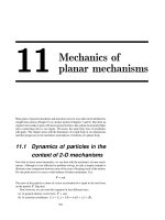
Introduction to
Flight Dynamics
Airplane Components "
Airplane Rotational
Degrees of Freedom"
Airplane Translational
Degrees of Freedom"
Axial Velocity"
Side Velocity"
Normal "
Velocity"
Phases of Flight"
Flight of a
Paper Airplane
Flight of a Paper Airplane
Example 1.3-1, Flight Dynamics"
• Red: Equilibrium
flight path"
• Black: Initial flight
path angle = 0"
• Blue: plus
increased initial
airspeed"
• Green: loop"
• Equations of
motion integrated
numerically to
estimate the flight
path"
Flight of a Paper Airplane
Example 1.3-1, Flight Dynamics"
• Red: Equilibrium
flight path"
• Black: Initial flight
path angle = 0"
• Blue: plus
increased initial
airspeed"
• Green: loop"
Assignment #2
•
Compute the trajectory of a balsa glider
Gliding Flight"
Configuration Aerodynamics"
Math Preliminaries
Notation for Scalars and Vectors "
• Scalar: usually lower case: a, b, c, …, x, y, z "
a =
2
−7
16
⎡
⎣
⎢
⎢
⎢
⎤
⎦
⎥
⎥
⎥
; x =
x
1
x
2
x
3
⎡
⎣
⎢
⎢
⎢
⎤
⎦
⎥
⎥
⎥
; y =
a
b
c
d
⎡
⎣
⎢
⎢
⎢
⎢
⎤
⎦
⎥
⎥
⎥
⎥
• Vector: usually bold or with underbar: x or x"
• Ordered set"
• Column of scalars"
• Dimension = n x 1"
a = 12; b = 7; c = a + b = 19; x = a + b
2
= 12 + 49 = 61
Matrices and Transpose"
x =
p
q
r
⎡
⎣
⎢
⎢
⎢
⎤
⎦
⎥
⎥
⎥
; A =
a b c
d e f
g h k
l m n
⎡
⎣
⎢
⎢
⎢
⎢
⎢
⎤
⎦
⎥
⎥
⎥
⎥
⎥
A
T
=
a d g l
b e h m
c f k n
⎡
⎣
⎢
⎢
⎢
⎤
⎦
⎥
⎥
⎥
x
T
= x
1
x
2
x
3
⎡
⎣
⎤
⎦
• Matrix: usually bold capital or capital: F or F"
• Dimension = (m x n)"
• Transpose: interchange rows and columns"
3 × 1
( )
4 × 3
( )
Multiplication "
ax
T
= ax
1
ax
2
ax
3
⎡
⎣
⎤
⎦
ax = xa =
ax
1
ax
2
ax
3
⎡
⎣
⎢
⎢
⎢
⎤
⎦
⎥
⎥
⎥
• Operands must be conformable"
• Multiplication of vector by scalar is associative, commutative, and
distributive"
• Could we add ?"
x + a
( )
• Only if"
dim x
( )
= 1 × 1
( )
a x + y
( )
= x + y
( )
a = ax + ay
( )
dim x
( )
= dim y
( )
Addition "
x =
a
b
⎡
⎣
⎢
⎤
⎦
⎥
; z =
c
d
⎡
⎣
⎢
⎤
⎦
⎥
• Conformable vectors and matrices are added term by
term "
x + z =
a + c
b + d
⎡
⎣
⎢
⎤
⎦
⎥
Inner Product "
x
T
x = x • x = x
1
x
2
x
3
⎡
⎣
⎤
⎦
x
1
x
2
x
3
⎡
⎣
⎢
⎢
⎢
⎤
⎦
⎥
⎥
⎥
• Inner (dot) product of vectors produces a scalar result"
(1 × m)(m × 1) = (1 × 1)
= (x
1
2
+ x
2
2
+ x
3
2
)
• Length (or magnitude) of
vector is square root of
dot product"
= (x
1
2
+ x
2
2
+ x
3
2
)
1/2
Vector Transformation "
y = Ax =
2 4 6
3 −5 7
4 1 8
−9 −6 −3
⎡
⎣
⎢
⎢
⎢
⎢
⎤
⎦
⎥
⎥
⎥
⎥
x
1
x
2
x
3
⎡
⎣
⎢
⎢
⎢
⎤
⎦
⎥
⎥
⎥
(n × 1) = (n × m)(m × 1)
• Matrix-vector product transforms one vector into another "
• Matrix-matrix product produces a new matrix"
=
2x
1
+ 4x
2
+ 6x
3
( )
3x
1
− 5x
2
+ 7x
3
( )
4 x
1
+ x
2
+ 8x
3
( )
−9x
1
− 6x
2
− 3x
3
( )
⎡
⎣
⎢
⎢
⎢
⎢
⎢
⎢
⎤
⎦
⎥
⎥
⎥
⎥
⎥
⎥
=
y
1
y
2
y
3
y
4
⎡
⎣
⎢
⎢
⎢
⎢
⎢
⎤
⎦
⎥
⎥
⎥
⎥
⎥
Derivatives and Integrals
of Vectors"
• Derivatives and integrals of vectors are vectors of
derivatives and integrals"
dx
dt
=
dx
1
dt
dx
2
dt
dx
3
dt
⎡
⎣
⎢
⎢
⎢
⎢
⎢
⎢
⎤
⎦
⎥
⎥
⎥
⎥
⎥
⎥
x
∫
dt =
x
1
∫
dt
x
2
∫
dt
x
3
∫
dt
⎡
⎣
⎢
⎢
⎢
⎢
⎢
⎤
⎦
⎥
⎥
⎥
⎥
⎥
Matrix Inverse"
x
y
z
⎡
⎣
⎢
⎢
⎢
⎤
⎦
⎥
⎥
⎥
2
=
cos
θ
0 − sin
θ
0 1 0
sin
θ
0 cos
θ
⎡
⎣
⎢
⎢
⎢
⎤
⎦
⎥
⎥
⎥
x
y
z
⎡
⎣
⎢
⎢
⎢
⎤
⎦
⎥
⎥
⎥
1
Transformation"
Inverse Transformation"
x
y
z
⎡
⎣
⎢
⎢
⎢
⎤
⎦
⎥
⎥
⎥
1
=
cos
θ
0 sin
θ
0 1 0
−sin
θ
0 cos
θ
⎡
⎣
⎢
⎢
⎢
⎤
⎦
⎥
⎥
⎥
x
y
z
⎡
⎣
⎢
⎢
⎢
⎤
⎦
⎥
⎥
⎥
2
x
2
= Ax
1
x
1
= A
−1
x
2
Matrix Identity and Inverse"
I
3
=
1 0 0
0 1 0
0 0 1
⎡
⎣
⎢
⎢
⎢
⎤
⎦
⎥
⎥
⎥
AA
−1
= A
−1
A = I
y = Iy
• Identity matrix: no change
when it multiplies a
conformable vector or matrix"
• A non-singular square matrix
multiplied by its inverse forms
an identity matrix"
AA
−1
=
cos
θ
0 −sin
θ
0 1 0
sin
θ
0 cos
θ
⎡
⎣
⎢
⎢
⎢
⎤
⎦
⎥
⎥
⎥
cos
θ
0 −sin
θ
0 1 0
sin
θ
0 cos
θ
⎡
⎣
⎢
⎢
⎢
⎤
⎦
⎥
⎥
⎥
−1
=
cos
θ
0 −sin
θ
0 1 0
sin
θ
0 cos
θ
⎡
⎣
⎢
⎢
⎢
⎤
⎦
⎥
⎥
⎥
cos
θ
0 sin
θ
0 1 0
−sin
θ
0 cos
θ
⎡
⎣
⎢
⎢
⎢
⎤
⎦
⎥
⎥
⎥
=
1 0 0
0 1 0
0 0 1
⎡
⎣
⎢
⎢
⎢
⎤
⎦
⎥
⎥
⎥
Dynamic Systems"
Dynamic Process: Current state depends on
prior state"
x "= dynamic state "
u "= input "
w "= exogenous disturbance"
p "= parameter"
t or k "= time or event index"
Observation Process: Measurement may
contain error or be incomplete"
y "= output (error-free)"
z "= measurement"
n "= measurement error"
• All of these quantities are vectors"
Sensors!
Actuators!
Mathematical Models of Dynamic
Systems are Differential Equations"
x(t )
dx(t )
dt
= f[x(t ),u(t ),w(t ),p(t ),t ]
y(t) = h[x(t),u(t)]
z(t ) = y(t ) + n(t)
Continuous-time dynamic process:
Vector Ordinary Differential Equation"
Output Transformation"
Measurement with Error"
dim x
( )
= n × 1
( )
dim f
( )
= n × 1
( )
dim u
( )
= m × 1
( )
dim w
( )
= s × 1
( )
dim p
( )
= l × 1
( )
dim y
( )
= r ×1
( )
dim h
( )
= r ×1
( )
dim z
( )
= r ×1
( )
dim n
( )
= r ×1
( )
Next Time:
Point-Mass Dynamics and
Aerodynamic/Thrust Forces
Reading:
Flight Dynamics
for Lecture 1: 1-27
for Lecture 2: 29-34, 38-53, 59-65, 103-107
Virtual Textbook
, Parts 1 and 2
Supplemental !
Material!
Ordinary Differential Equations"
dx(t )
dt
= f x(t ),u(t ),w(t )
[ ]
dx(t )
dt
= f x(t ),u(t ),w(t ),p(t ),t
[ ]
dx(t )
dt
= F(t)x(t ) + G(t)u(t ) + L(t)w(t )
dx(t )
dt
= Fx(t ) + G u(t ) + L w(t )
Examples of Airplane Dynamic
System Models"
• Nonlinear, Time-Varying"
– Large amplitude motions"
– Significant change in mass"
• Nonlinear, Time-Invariant"
– Large amplitude motions"
– Negligible change in mass"
• Linear, Time-Varying"
– Small amplitude motions"
– Perturbations from a dynamic
flight path"
• Linear, Time-Invariant"
– Small amplitude motions"
– Perturbations from an
equilibrium flight path"
Simplified Longitudinal Modes of Motion"
Phugoid (Long-Period) Mode"
Airspeed! Flight Path Angle!
Pitch Rate! Angle of Attack!
Short-Period Mode"
Airspeed! Flight Path Angle!
Pitch Rate! Angle of Attack!
• Note change in
time scale"
Simplified Longitudinal Modes of Motion"
Simplified Lateral Modes of Motion"
Dutch-Roll Mode"
Yaw Rate!
Sideslip Angle!
Roll and Spiral Modes"
Roll Rate! Roll Angle!
Simplified Lateral Modes of Motion"
Flight Dynamics Book and
Computer Code"
• All programs are accessible from the Flight Dynamics web
page"
– />• or directly"
• Errata for the book are listed there"
• 6-degree-of-freedom nonlinear simulation of a business jet
aircraft (MATLAB)"
– />• Linear system analysis (MATLAB)"
– />• Paper airplane simulation (MATLAB)"
– />• Performance analysis of a business jet aircraft (Excel)"
– />Helpful Resources"
• Web pages"
– />– />– />• Princeton University Engineering Library (paper and on-
line)"
– />• NACA/NASA and AIAA pubs"
– />Primary Learning Objectives
!
Introduction to the performance, stability, and control of
fixed-wing aircraft ranging from micro-uninhabited air
vehicles through general aviation, jet transport, and fighter
aircraft to re-entry vehicles.
!
Understanding of aircraft equations of motion,
configuration aerodynamics, and methods for analysis of
linear and nonlinear systems.
!
Appreciation of the historical context within which past
aircraft have been designed and operated, providing a sound
footing for the development of future aircraft.
More Learning Objectives"
! Detailed evaluation of the linear and nonlinear flight characteristics of a
specific aircraft type."
! Improved skills for presenting ideas, orally and on paper."
! Improved ability to analyze complex, integrated problems."
! Demonstrated computing skills, through thorough knowledge and
application of MATLAB."
! Facility in evaluating aircraft kinematics and dynamics, flight envelopes, trim
conditions, maximum range, climbing/diving/turning flight, inertial properties,
stability-and-control derivatives, longitudinal and lateral-directional transients,
transfer functions, state-space models, and frequency response."