Microsoft SQL Server 2008 R2 Unleashed- P84 ppsx

ptg
774
CHAPTER 24 Creating and Managing Tables
the foreign key constraints that reference a table. Listing 24.18 shows an execution of this
stored procedure for the Sales.Store table in the AdventureWorks2008 database. The
procedure results include information about all the constraints on the table. The results to
focus on are those that follow the heading Table Is Referenced by Foreign Key. The partial
results shown in Listing 24.18 for the Sales.Store table indicate that
FK_StoreContact_Store_CustomerID must be dropped first before you can drop the
Sales.Store table.
LISTING 24.18 Using sp_helpconstraint to Find Foreign Key References
sp_helpconstraint [Sales.Store]
/*partial results of sp_helpconstraint execution
Table is referenced by foreign key

AdventureWorks2008.Sales.StoreContact: FK_StoreContact_Store_CustomerID
*/
Two other approaches are useful for identifying foreign key references prior to dropping a
table. The first is using a database diagram. You can create a new database diagram and
add the table that you are considering for deletion. After the table is added, you right-click
the table in Object Explorer and select Add Related Tables. The related tables, including
those that have foreign key references, are then added. You can then right-click the rela-
tionship line connecting two tables and select Delete Relationships from Database. When
you have deleted all the foreign key relationships from the diagram, you can right-click
the table you want to delete and select Generate Change Script to create a script that can
be used to remove the foreign key relationship(s).
The other approach is to right-click the table in Object Explorer and choose View
Dependencies. The dialog that appears gives you the option of viewing the objects that
depend on the table or viewing the objects on which the table depends. If you choose the
option to view the objects that depend on the table, all the dependent objects are
displayed, but you can focus on the objects that are tables.

Using Partitioned Tables
In SQL Server 2008, tables are stored in one or more partitions. Partitions are organiza-
tional units that allow you to divide data into logical groups. By default, a table has only a
single partition that contains all the data. The power of partitions comes into play when
you define multiple partitions for a table that is segmented based on a key column. This
column allows the data rows to be horizontally split. For example, a date/time column can
be used to divide each month’s data into a separate partition. These partitions can also be
aligned to different filegroups for added flexibility, ease of maintenance, and improved
performance.
Download from www.wowebook.com
ptg
775
Using Partitioned Tables
24
The important point to remember is that you access tables with multiple partitions (which
are called partitioned tables) the same way you access tables with a single partition. Data
Manipulation Language (DML) operations such as INSERT and SELECT statements reference
the table the same way, regardless of partitioning. The difference between these types of
tables has to do with the back-end storage and the organization of the data.
Generally, partitioning is most useful for large tables. Large is a relative term, but these
tables typically contain millions of rows and take up gigabytes of space. Often, the tables
targeted for partitioning are large tables experiencing performance problems because of
their size. Partitioning has several different applications, including the following:
. Archival—Table partitions can be moved from a production table to another
archive table that has the same structure. When done properly, this partition move-
ment is very fast and allows you to keep a limited amount of recent data in the
production table while keeping the bulk of the older data in the archive table.
. Maintenance—Table partitions that have been assigned to different filegroups can
be backed up and maintained independently of each other. With very large tables,
maintenance activities on the entire table (such as backups) can take a prohibitively

long time. With partitioned tables, these maintenance activities can be performed at
the partition level. Consider, for example, a table that is partitioned by month: all
the new activity (updates and insertions) occurs in the partition that contains the
current month’s data. In this scenario, the current month’s partition would be the
focus of the maintenance, thus limiting the amount of data you need to process.
. Query performance—Partitioned tables joined on partitioned columns can experi-
ence improved performance because the Query Optimizer can join to the table based
on the partitioned column. The caveat is that joins across partitioned tables not
joining on the partitioned column may actually experience some performance degra-
dation. Queries can also be parallelized along the partitions.
Now that we have discussed some of the reasons to use partitioned tables, let’s look at
how to set up partitions. There are three basic steps:
1. Create a partition function that maps the rows in the table to partitions based on
the value of a specified column.
2. Create a partition scheme that outlines the placement of the partitions in the parti-
tion function to filegroups.
3. Create a table that utilizes the partition scheme.
These steps are predicated on a good partitioning design, based on an evaluation of the
data within the table and the selection of a column that will effectively split the data. If
multiple filegroups are used, those filegroups must also exist before you execute the three
steps in partitioning. The following sections look at the syntax related to each step, using
simple examples. These examples utilize the
BigPubs2008 database.
Download from www.wowebook.com
ptg
776
CHAPTER 24 Creating and Managing Tables
Creating a Partition Function
A partition function identifies values within a table that will be compared to the column
on which you partition the table. As mentioned previously, it is important that you know

the distribution of the data and the specific range of values in the partitioning column
before you create the partition function. The following query provides an example of
determining the distribution of data values in the sales_big table by year:
Select the distinct yearly values
SELECT year(ord_date) as ‘year’, count(*) ‘rows’
FROM sales_big
GROUP BY year(ord_date)
ORDER BY 1
go
year rows

2005 30
2006 613560
2007 616450
2008 457210
You can see from the results of the SELECT statement that there are four years’ worth of
data in the sales_big table. Because the values specified in the CREATE PARTITION FUNC-
TION statement are used to establish data ranges, at a minimum, you would need to
specify at least three data values when defining the partition function, as shown in the
following example:
Create partition function with the yearly values to partition the data
CREATE PARTITION FUNCTION SalesBigPF1 (datetime)
AS RANGE RIGHT FOR VALUES
(‘01/01/2006’, ‘01/01/2007’,
‘01/01/2008’)
GO
In this example, four ranges, or partitions, would be established by the three RANGE RIGHT
values specified in the statement:
. values < 01/01/2006—This partition includes any rows prior to 2006.
. values >= 01/01/2006 AND values < 01/01/2007—This partition includes

all rows for 2006.
. values >= 01/01/2007 AND values < 01/01/2008—This partition includes
all rows for 2007.
. values > 01/01/2008—This includes any rows for 2008 or later.
This method of partitioning would be more than adequate for a static table that is not
going to be receiving any additional data rows for different years than already exist in the
Download from www.wowebook.com
ptg
777
Using Partitioned Tables
24
table. However, if the table is going to be populated with additional data rows after it has
been partitioned, it is good practice to add additional range values at the beginning and
end of the ranges to allow for the insertion of data values less than or greater than the
existing range values in the table. To create these additional upper and lower ranges, you
would want to specify five values in the VALUES clause of the CREATE PARTITION FUNCTION,
as shown in Listing 24.19. The advantages of having these additional partitions are
demonstrated later in this section.
LISTING 24.19 Creating a Partition Function
if exists (select 1 from sys.partition_functions where name = ‘SalesBigPF1’)
drop partition function SalesBigPF1
go
Create partition function with the yearly values to partition the data
Create PARTITION FUNCTION SalesBigPF1 (datetime)
AS RANGE RIGHT FOR VALUES
(‘01/01/2005’, ‘01/01/2006’, ‘01/01/2007’,
‘01/01/2008’, ‘01/01/2009’)
GO
In this example, six ranges, or partitions, are established by the five range values specified in
the statement:

. values < 01/01/2005—This partition includes any rows prior to 2005.
. values >= 01/01/2005 AND values < 01/01/2006—This partition includes
all rows for 2005.
. values >= 01/01/2006 AND values < 01/01/2007—This partition includes
all rows for 2006.
. values >= 01/01/2007 AND values < 01/01/2008—This partition includes
all rows for 2007.
. values >= 01/01/2008 AND values < 01/01/2009—This partition includes
all rows for 2008.
. values >= 01/01/2009—This partition includes any rows for 2009 or later.
An alternative to the RIGHT clause in the CREATE PARTITION FUNCTION statement is the
LEFT clause. The LEFT clause is similar to RIGHT, but it changes the ranges such that the <
operands are changed to <=, and the >= operands are changed to >.
TIP
Using RANGE RIGHT partitions for datetime values is usually best because this
approach makes it easier to specify the limits of the ranges. The datetime data type
can store values only with accuracy to 3.33 milliseconds. The largest value it can store
is 0.997 milliseconds. A value of 0.998 milliseconds rounds down to 0.997, and a
value of 0.999 milliseconds rounds up to the next second.
Download from www.wowebook.com
ptg
778
CHAPTER 24 Creating and Managing Tables
If you used a RANGE LEFT partition, the maximum time value you could include with the
year to get all values for that year would be 23:59:59.997. For example, if you speci-
fied 12/31/2006 23:59:59.999 as the boundary for a RANGE LEFT partition, it would
be rounded up so that it would also include rows with datetime values less than or
equal to 01/01/2007 00:00:00.000, which is probably not what you would want. You
would redefine the example shown in Listing 24.19 as a RANGE LEFT partition function
as follows:

CREATE PARTITION FUNCTION SalesBigPF1 (datetime)
AS RANGE LEFT FOR VALUES
(‘12/31/2004 23:59:59.997’, ‘12/31/2005 23:59:59.997’,
‘12/31/2006 23:59: 59.997’, ‘12/31/2007 23:59:59.997’,
‘12/31/2008 23:59:59.997’)
As you can see, it’s a bit more straightforward and probably less confusing to use
RANGE RIGHT partition functions when dealing with datetime values or any other con-
tinuous-value data types, such as float or numeric.
Creating a Partition Scheme
After you create a partition function, the next step is to associate a partition scheme with
the partition function. A partition scheme can be associated with only one partition func-
tion, but a partition function can be shared across multiple partition schemes.
The core function of a partition scheme is to map the values defined in the partition func-
tion to filegroups. When creating the statement for a partition scheme, you need to keep
in mind the following:
. A single filegroup can be used for all partitions, or a separate filegroup can be used
for each individual partition.
. Any filegroup referenced in the partition scheme must exist before the partition
scheme is created.
. There must be enough filegroups referenced in the partition scheme to accommo-
date all the partitions. The number of partitions is one more than the number of
values specified in the partition function.
. The number of partitions is limited to 1,000.
. The filegroups listed in the partition scheme are assigned to the partitions defined in
the function based on the order in which the filegroups are listed.
Listing 24.20 creates a partition schema that references the partition function created in
Listing 24.19. This example assumes that the referenced filegroups have been created for
each of the partitions. (For more information on creating filegroups and secondary files,
see Chapter 23.)
Download from www.wowebook.com

ptg
779
Using Partitioned Tables
24
NOTE
If you would like to create the same filegroups and files used by the examples in this
section, check out the script file called Create_Filegroups_and_Files_for_
Partitioning.sql on the included CD in the code listings directory for this chapter. If
you run this script, it creates all the necessary file groups and files referenced in the
examples. Note that you need to edit the script to change the FILENAME value if you
need the files to be created in a directory other than C:\MSSQL2008\DATA.
LISTING 24.20 Creating a Partition Scheme
Create a partition scheme that is aligned with the partition function
CREATE PARTITION SCHEME SalesBigPS1
AS PARTITION SalesBigPF1
TO ([Older_data], [2005_data], [2006_data],
[2007_data], [2008_data], [2009_data])
GO
Alternatively, if all partitions are going to be on the same filegroup, such as the PRIMARY
filegroup, you could use the following:
Create PARTITION SCHEME SalesBigPS1
as PARTITION SalesBigPF1
ALL to ([PRIMARY])
go
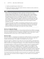
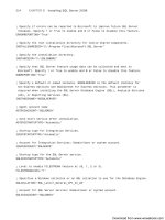
Notice that SalesBigPF1 is referenced as the partition function in Listing 24.20. This ties
together the partition scheme and partition function. Figure 24.7 shows how the parti-
tions defined in the function would be mapped to the filegroup(s). At this point, you have
made no changes to any table, and you have not even specified the column in the table
that you will partition. The next section discusses those details.
Creating a Partitioned Table

Tables are partitioned only when they are created. This is an important point to keep in
mind when you are considering adding partitions to a table that already exists.
Sometimes, performance issues or other factors may lead you to determine that a table
you have already created and populated may benefit from being partitioned.
The re-creation of large tables in a production environment requires some forethought
and planning. The data in the table must be retained in another location for you to re-
create the table. Bulk copying the data to a flat file and renaming the table are two possi-
ble solutions for retaining the data. After you determine the data retention method, you
can re-create the table, with the new partition scheme. For simplicity’s sake, the example
in Listing 24.21 creates a new table named sales_big_Partitioned instead of using the
Download from www.wowebook.com
ptg
780
CHAPTER 24 Creating and Managing Tables
1996_data
Filegroup
1996_data
Filegroup
Older_data
Filegroup
1992_data
Filegroup
1993_data
Filegroup
1994_data
Filegroup
1995_data
Filegroup
Boundary
1

Boundary
2
Boundary
3
Partition Scheme
Boundary
4
Boundary
5
1992-01-01 1993-01-01 1994-01-01 1995-01-01 1996-01-01
1
Partition #
2 3 4 5 6
1991 and
Earlier Data
1992 Data 1993 Data 1994 Data 1995 Data 1996 Data
Later Data
FIGURE 24.7 Mapping of partitions to filegroups, using a RANGE RIGHT partition function.
original sales_big table. The second part of Listing 24.21 copies the data from the
sales_big table into the sales_big_Partitioned table.
LISTING 24.21 Creating a Partitioned Table
CREATE TABLE dbo.sales_big_Partitioned(
sales_id int IDENTITY(1,1) NOT NULL,
stor_id char(4) NOT NULL,
ord_num varchar(20) NOT NULL,
ord_date datetime NOT NULL,
qty smallint NOT NULL,
payterms varchar(12) NOT NULL,
title_id dbo.tid NOT NULL
) ON SalesBigPS1 (ord_date) this statement is key to Partitioning the table

GO
GO
Insert data from the sales_big table into the new sales_big_partitioned table
SET IDENTITY_INSERT sales_big_Partitioned ON
GO
INSERT sales_big_Partitioned with (TABLOCKX)
(sales_id, stor_id, ord_num, ord_date, qty, payterms, title_id)
SELECT sales_id, stor_id, ord_num, ord_date, qty, payterms, title_id
FROM sales_big
Download from www.wowebook.com
ptg
781
Using Partitioned Tables
24
go
SET IDENTITY_INSERT sales_big_Partitioned OFF
GO
The key clause to take note of in this listing is ON SalesBigPS1 (ord_date). This clause
identifies the partition scheme on which to create the table (SalesBigPS1) and the column
within the table to use for partitioning (ord_date).
After you create the table, you might wonder whether the table was partitioned correctly.
Fortunately, there are some catalog views related to partitions that you can query for this
kind of information. Listing 24.22 shows a sample SELECT statement that utilizes the
sys.partitions view. The results of the statement execution are shown immediately after
the SELECT statement. Notice that there are six numbered partitions and that the esti-
mated number of rows for each partition corresponds to the number of rows you saw
when you selected the data from the unpartitioned SalesBig table.
LISTING 24.22 Viewing Partitioned Table Information
select convert(varchar(16), ps.name) as partition_scheme,
p.partition_number,

convert(varchar(10), ds2.name) as filegroup,
convert(varchar(19), isnull(v.value, ‘’), 120) as range_boundary,
str(p.rows, 9) as rows
from sys.indexes i
join sys.partition_schemes ps on i.data_space_id = ps.data_space_id
join sys.destination_data_spaces dds
on ps.data_space_id = dds.partition_scheme_id
join sys.data_spaces ds2 on dds.data_space_id = ds2.data_space_id
join sys.partitions p on dds.destination_id = p.partition_number
and p.object_id = i.object_id and p.index_id = i.index_id
join sys.partition_functions pf on ps.function_id = pf.function_id
LEFT JOIN sys.Partition_Range_values v on pf.function_id = v.function_id
and v.boundary_id = p.partition_number - pf.boundary_value_on_right
WHERE i.object_id = object_id(‘sales_big_partitioned’)
and i.index_id in (0, 1)
order by p.partition_number
/* Results from the previous SELECT statement
partition_scheme partition_number filegroup range_boundary rows

SalesBigPS1 1 Older_Data 0
SalesBigPS1 2 2005_Data 2005-01-01 00:00:00 30
SalesBigPS1 3 2006_Data 2006-01-01 00:00:00 613560
SalesBigPS1 4 2007_Data 2007-01-01 00:00:00 616450
SalesBigPS1 5 2008_Data 2008-01-01 00:00:00 457210
SalesBigPS1 6 2009_Data 2009-01-01 00:00:00 0
*/
Download from www.wowebook.com
ptg
782
CHAPTER 24 Creating and Managing Tables

Adding and Dropping Table Partitions
One of the most useful features of partitioned tables is that you can add and drop entire
partitions of table data in bulk. If the table partitions are set up properly, these commands
can take place in seconds, without the expensive input/output (I/O) costs of physically
copying or moving the data. You can add and drop table partitions by using the SPLIT
RANGE and MERGE RANGE options of the ALTER PARTITION FUNCTION command:
ALTER PARTITION FUNCTION partition_function_name()
{ SPLIT RANGE ( boundary_value ) | MERGE RANGE ( boundary_value ) }
Adding a Table Partition
The SPLIT RANGE option adds a new boundary point to an existing partition function and
affects all objects that use this partition function. When this command is run, one of the
function partitions is split in two. The new partition is the one that contains the new
boundary point. The new partition is created to the right of the boundary value if the
partition is defined as a RANGE RIGHT partition function or to the left of the boundary if it
is a RANGE LEFT partition function. If the partition is empty, the split is instantaneous.
If the partition being split contains data, any data on the new side of the boundary is
physically deleted from the old partition and inserted into the new partition. In addition
to being I/O intensive, a split is also log intensive, generating log records that are four
times the size of the data being moved. In addition, an exclusive table lock is held for the
duration of the split. If you want to avoid this costly overhead when adding a new parti-
tion to the end of the partition range, it is recommended that you always keep an empty
partition available at the end and split it before it is populated with data. If the partition
is empty, SQL Server does not need to scan the partition to see whether there is any data
to be moved.
NOTE
Avoiding the overhead associated with splitting a partition is the reason the code in
Listing 24.19 defined the SalesBigPF1 partition function with a partition for 2009,
even though there is no 2009 data in the sales_big_partitioned table. As long as
you split the partition before any 2009 data is inserted into the table and the 2009
partition is empty, no data needs to be moved, so the split is instantaneous.

Before you split a partition, a filegroup must be marked to be the NEXT USED partition by
the partition scheme that uses the partition function. You initially allocate filegroups to
partitions by using a CREATE PARTITION SCHEME statement. If a CREATE PARTITION SCHEME
statement allocates more filegroups than there are partitions defined in the CREATE PARTI-
TION FUNCTION statement, one of the unassigned filegroups is automatically marked as
NEXT USED by the partition scheme, and it will hold the new partition.
Download from www.wowebook.com
ptg
783
Using Partitioned Tables
24
If there are no filegroups currently marked NEXT USED by the partition scheme, you must
use ALTER PARTITION SCHEME to either add a filegroup or designate an existing filegroup to
hold the new partition. This can be a filegroup that already holds existing partitions. Also,
if a partition function is used by more than one partition scheme, all the partition schemes
that use the partition function to which you are adding partitions must have a NEXT USED
filegroup. If one or more do not have a NEXT USED filegroup assigned, the ALTER PARTITION
FUNCTION statement fails, and the error message displays the partition scheme or schemes
that lack a NEXT USED filegroup.
The following SQL statement adds a NEXT USED filegroup to the SalesBigPS1 partition
scheme. Note that in this example, the filegroup specified is a new filegroup, 2010_DATA:
ALTER PARTITION SCHEME SalesBigPS1 NEXT USED ‘2010_Data’
Now that you have specified a NEXT USED filegroup for the partition scheme, you can go
ahead and add the new range for 2010 and later data rows to the partition function, as in
the following example:
Alter partition function with the yearly values to partition the data
ALTER PARTITION FUNCTION SalesBigPF1 () SPLIT RANGE (‘01/01/2010’)
GO
Figure 24.8 shows the effects of splitting the 2009 table partition.
You can also see the effects of splitting the partition on the system catalogs by running

the same query as shown earlier, in Listing 24.22:
Boundary
6
Added
1997-01-01
Boundary
1
Boundary
2
Boundary
3
Boundary
4
Boundary
5
1992-01-01 1993-01-01 1994-01-01 1995-01-01 1996-01-01
1 2 3 4 5 76
1991 and
Earlier Data
1992 Data 1993 Data 1994 Data 1995 Data 1996 Data
1997 and
Later Data
Any 1997 and later
data will be moved
FIGURE 24.8 The effects of splitting a RANGE RIGHT table partition.
Download from www.wowebook.com