Microsoft SQL Server 2008 R2 Unleashed- P85 pptx

ptg
784
CHAPTER 24 Creating and Managing Tables
/* New results from the SELECT statement in Listing 24.22
partition_scheme partition_number filegroup range_boundary rows

SalesBigPS1 1 Older_Data 0
SalesBigPS1 2 2005_Data 2005-01-01 00:00:00 30
SalesBigPS1 3 2006_Data 2006-01-01 00:00:00 613560
SalesBigPS1 4 2007_Data 2007-01-01 00:00:00 616450
SalesBigPS1 5 2008_Data 2008-01-01 00:00:00 457210
SalesBigPS1 6 2009_Data 2009-01-01 00:00:00 0
SalesBigPS1 7 2010_Data 2010-01-01 00:00:00 0
*/
Dropping a Table Partition
You can drop a table partition by using the ALTER PARTITION FUNCTION MERGE RANGE
command. This command essentially removes a boundary point from a partition function
as the partitions on each side of the boundary are merged into one. The partition that held
the boundary value is removed. The filegroup that originally held the boundary value is
removed from the partition scheme unless it is used by a remaining partition or is marked
with the NEXT USED property.
Any data that was in the removed partition is moved to the remaining neighboring parti-
tion. If a RANGE RIGHT partition boundary was removed, the data that was in that bound-
ary’s partition is moved to the partition to the left of boundary. If it was a RANGE LEFT
partition, the data is moved to the partition to the right of the boundary.
The following command merges the 2005 partition into the Old_Data partition for the
sales_big_partitioned table:
ALTER PARTITION FUNCTION SalesBigPF1 () MERGE RANGE (‘01/01/2005’)
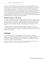
Figure 24.9 demonstrates how the 2005 RANGE RIGHT partition boundary is removed and
the data is merged to the left, into the Old_Data partition.
CAUTION

Splitting or merging partitions for a partition function affects all objects using that parti-
tion function.
You can also see the effects of merging the partition on the system catalogs by running
the same query as shown in Listing 24.22:
/* New results from the SELECT statement in Listing 24.20
partition_scheme partition_number filegroup range_boundary rows

SalesBigPS1 1 Older_Data 30
SalesBigPS1 3 2006_Data 2006-01-01 00:00:00 613560
Download from www.wowebook.com
ptg
785
Using Partitioned Tables
24
Boundary
6
Boundary
1
Removed
Boundary
2
Boundary
3
Boundary
4
Boundary
5
1992-01-01 1993-01-01 1994-01-01 1995-01-01 1996-01-01 1996-07-01
1 2 3 4 5 76
1991 and

Earlier Data
1992 Data 1993 Data 1994 Data 1995 Data 1996 Data
1997 and
Later Data
1992 Data
Moved
FIGURE 24.9 The effects of merging a RANGE RIGHT table partition.
Like the split operation, the merge operation occurs instantaneously if the partition being
merged is empty. The process can be very I/O intensive if the partition has a large
amount of data in it. Any rows in the removed partition are physically moved into the
remaining partition. This operation is also very log intensive, requiring log space approxi-
mately four times the size of data being moved. An exclusive table lock is held for the
duration of the merge.
If you no longer want to keep the data in the table for a partition you are merging, you
can move the data in the partition to another empty table or empty table partition by
using the SWITCH PARTITION option of the ALTER TABLE command. This option is
discussed in more detail in the following section.
Switching Table Partitions
One of the great features of table partitions is that they enable you to instantly swap the
contents of one partition to an empty table, the contents from a partition on one table to
a partition in another table, or an entire table’s contents into another table’s empty parti-
tion. This operation performs changes only to metadata in the system catalogs for the
affected tables/partitions, with no actual physical movement of data.
SalesBigPS1 4 2007_Data 2007-01-01 00:00:00 616450
SalesBigPS1 5 2008_Data 2008-01-01 00:00:00 457210
SalesBigPS1 6 2009_Data 2009-01-01 00:00:00 0
SalesBigPS1 7 2010_Data 2010-01-01 00:00:00 0
*/
Download from www.wowebook.com
ptg

786
CHAPTER 24 Creating and Managing Tables
For you to switch data from a partition to a table or from a table into a partition, the
following criteria must be met:
. The source table and target table must both have the same structure (that is, the
same columns in the same order, with the same names, data types, lengths, preci-
sions, scales, nullabilities, and collations). The tables must also have the same
primary key constraints and settings for ANSI_NULLS and QUOTED_IDENTIFIER.
. The source and target of the ALTER TABLE SWITCH statement must reside in the
same filegroup.
. If you are switching a partition to a single, nonpartitioned table, the table receiving
the partition must already be created, and it must be empty.
. If you are adding a table as a partition to an already existing partitioned table or
moving a partition from one partitioned table to another, the receiving partition
must exist, and it must be empty.
. If you are switching a partition from one partitioned table to another, both tables
must be partitioned on the same column.
. The source must have all the same indexes as the target, and the indexes must also
be in the same filegroup.
. If you are switching a nonpartitioned table to a partition of an already existing parti-
tioned table, the nonpartitioned table must have a constraint defined on the column
corresponding to the partition key of the target table to ensure that the range of
values fits within the boundary values of the target partition.
. If the target table has any
FOREIGN KEY constraints, the source table must have the
same foreign keys defined on the corresponding columns, and those foreign keys
must reference the same primary keys that the target table references.
If you are switching a partition of a partitioned table to another partitioned table, the
boundary values of the source partition must fit within those of the target partition. If the
boundary values do not fit, a constraint must be defined on the partition key of the

source table to make sure all the data in the table fits into the boundary values of the
target partition.
CAUTION
If the tables have IDENTITY columns, partition switching can result in the introduction
of duplicate values in IDENTITY columns of the target table and gaps in the values of
IDENTITY columns in the source table. You can use DBCC_CHECKIDENT to check the
identity values of tables and correct them if necessary.
When you switch a partition, data is not physically moved. Only the metadata informa-
tion in the system catalogs indicating where the data is stored is changed. In addition, all
associated indexes are automatically switched, along with the table or partition.
Download from www.wowebook.com
ptg
787
Using Partitioned Tables
24
To switch table partitions, you use the ALTER TABLE command:
ALTER TABLE table_name SWITCH [ PARTITION source_partition_number_expression ]
TO target_table [ PARTITION target_partition_number_expression ]
You can use the ALTER TABLE SWITCH command to switch an unpartitioned table into a
table partition, switch a table partition into an empty unpartitioned table, or switch a
table partition into another table’s empty table partition. The code shown in Listing 24.23
creates a table to hold the data from the 2006 partition and then switches the 2006 parti-
tion from the sales_big_partitioned table to the new table.
LISTING 24.23 Switching a Partition to an Empty Table
CREATE TABLE dbo.sales_big_2006(
sales_id int IDENTITY(1,1) NOT NULL,
stor_id char(4) NOT NULL,
ord_num varchar(20) NOT NULL,
ord_date datetime NOT NULL,
qty smallint NOT NULL,

payterms varchar(12) NOT NULL,
title_id dbo.tid NOT NULL
) ON ‘2006_data’ required in order to switch the partition to this table
go
alter table sales_big_partitioned
switch partition $PARTITION.SalesBigPF1 (‘1/1/2006’)
to sales_big_2006
go
Note that Listing 24.23 uses the $PARTITION function. You can use this function with any
partition function name to return the partition number that corresponds with the speci-
fied partitioning column value. This prevents you from having to query the system cata-
logs to determine the specific partition number for the specified partition value.
You can run the query from Listing 24.22 to show that the 2006 partition is now empty:
partition_scheme partition_number filegroup range_boundary rows

SalesBigPS1 1 Older_Data 30
SalesBigPS1 2 2006_Data 2006-01-01 00:00:00 0
SalesBigPS1 3 2007_Data 2007-01-01 00:00:00 616450
SalesBigPS1 4 2008_Data 2008-01-01 00:00:00 457210
SalesBigPS1 5 2009_Data 2009-01-01 00:00:00 0
SalesBigPS1 6 2010_Data 2010-01-01 00:00:00 0
Download from www.wowebook.com
ptg
788
CHAPTER 24 Creating and Managing Tables
Now that the 2006 data partition is empty, you can merge the partition without incurring
the I/O cost of moving the data to the Older_data partition:
ALTER PARTITION FUNCTION SalesBigPF1 () merge RANGE (‘1/1/2006’)
Rerunning the query in Listing 24.22 now returns the following result set:
partition_scheme partition_number filegroup range_boundary rows

SalesBigPS1 1 Older_Data 30
SalesBigPS1 2 2007_Data 2007-01-01 00:00:00 616450
SalesBigPS1 3 2008_Data 2008-01-01 00:00:00 457210
SalesBigPS1 4 2009_Data 2009-01-01 00:00:00 0
SalesBigPS1 5 2010_Data 2010-01-01 00:00:00 0
To demonstrate switching a table into a partition, you can update the date for all the rows
in the sales_big_2006 table to 2009 and switch it into the 2009 partition of the
sales_big_partitioned table. Note that before you can do this, you need to copy the data
to a table in the 2009_data filegroup and also put a check constraint on the ord_date
column to make sure all rows in the table are limited to values that are valid for the
2009_data partition. Listing 24.24 shows the commands you use to create the new table
and switch it into the 2009 partition of the sales_big_partitioned table.
LISTING 24.24 Switching a Table to an Empty Partition
CREATE TABLE dbo.sales_big_2009(
sales_id int IDENTITY(1,1) NOT NULL,
stor_id char(4) NOT NULL,
ord_num varchar(20) NOT NULL,
ord_date datetime NOT NULL
constraint CK_sales_big_2009_ord_date
check (ord_date >= ‘1/1/2009’ and ord_date < ‘1/1/2010’),
qty smallint NOT NULL,
payterms varchar(12) NOT NULL,
title_id dbo.tid NOT NULL
) ON ‘2009_data’ required to switch the table to the 2009 partition
go
set identity_insert sales_big_2009 on
go
insert sales_big_2009 (sales_id, stor_id, ord_num,
ord_date, qty, payterms, title_id)

select sales_id, stor_id, ord_num,
dateadd(yy, 3, ord_date),
qty, payterms, title_id
from sales_big_2006
go
set identity_insert sales_big_2009 off
Download from www.wowebook.com
ptg
789
Creating Temporary Tables
24
go
alter table sales_big_2009
switch to sales_big_partitioned
partition $PARTITION.SalesBigPF1 (‘1/1/2009’)
go
Rerunning the query from Listing 24.22 now returns the following result:
partition_scheme partition_number filegroup range_boundary rows

SalesBigPS1 1 Older_Data 30
SalesBigPS1 2 2007_Data 2007-01-01 00:00:00 616450
SalesBigPS1 3 2008_Data 2008-01-01 00:00:00 457210
SalesBigPS1 4 2009_Data 2009-01-01 00:00:00 613560
SalesBigPS1 5 2010_Data 2010-01-01 00:00:00 0
TIP
Switching data into or out of partitions provides a very efficient mechanism for archiv-
ing old data from a production table, importing new data into a production table, or
migrating data to an archive table. You can use SWITCH to empty or fill partitions very
quickly. As you’ve seen in this section, split and merge operations occur instantaneous-
ly if the partitions being split or merged are empty first. If you must split or merge par-

titions that contain a lot of data, you should empty them first by using SWITCH before
you perform the split or merge.
Creating Temporary Tables
A temporary table is a special type of table that is automatically deleted when it is no
longer used. Temporary tables have many of the same characteristics as permanent tables
and are typically used as work tables that contain intermediate results.
You designate a table as temporary in SQL Ser ver by prefacing the table name with a single
pound sign (#) or two pound signs (##). Temporary tables are created in tempdb; if a
temporary table is not explicitly dropped, it is dropped when the session that created it
ends or the stored procedure it was created in finishes execution.
If a table name is prefaced with a single pound sign (for example, #table1), it is a private
temporary table, available only to the session that created it.
A table name prefixed with a double pound sign (for example, ##table2) indicates that it is
a global temporary table, which means it is accessible by all database connections. A global
temporary table exists until the session that created it terminates. If the creating session
terminates while other sessions are accessing the table, the temporary table is available to
those sessions until the last session’s query ends, at which time the table is dropped.
Download from www.wowebook.com
ptg
790
CHAPTER 24 Creating and Managing Tables
A common way of creating a temporary table is to use the SELECT INTO method as shown
in the following example:
SELECT* INTO #Employee2 FROM Employee
This method creates a temporary table with a structure like the table that is being selected
from. It also copies the data from the original table and inserts it into this new temporary
table. All of this is done with this one simple command.
NOTE
Table variable s are a good alter na tive to tem porar y tables. These variables are also
temporary in nature and have some advantages over temporary tables. Table variables

are easy to create, are automatically deleted, cause fewer recompilations, and use fewer
locking and logging resources. Generally speaking, you should consider using table vari-
ables instead of temporary tables when the temporary results are relatively small.
Parallel query plans are not generated with table variables, and this can impede overall
performance when you are accessing a table variable that has a large number of rows.
For more information on using temporary tables and table variables, see Chapter 43,
“Transact-SQL Programming Guidelines, Tips, and Tricks,” that is found on the bonus CD.
Tables created without the # prefix but explicitly created in tempdb are also considered
temporary, but they are a more permanent form of a temporary table. They are not
dropped automatically until SQL Server is restarted and tempdb is reinitialized.
Summary
Tables are the key to a relational database system. When you create tables, you need to
pay careful attention to choosing the proper data types to ensure efficient storage of data,
adding appropriate constraints to maintain data integrity, and scripting the creation and
modification of tables to ensure that they can be re-created, if necessary.
Good table design includes the creation of indexes on a table. Tables without indexes are
generally inefficient and cause excessive use of resources on your database server. Chapter
25, “Creating and Managing Indexes,” covers indexes and their critical role in effective
table design.
Download from www.wowebook.com
ptg
CHAPTER 25
Creating and Managing
Indexes
IN THIS CHAPTER
. What’s New in Creating and
Managing Indexes
. Ty pes of Indexes
. Creating Indexes
. Managing Indexes

. Dropping Indexes
. Online Indexing Operations
. Indexes on Views
Just like the index in this book, an index on a table or
view allows you to efficiently find the information you are
looking for in a database. SQL Server does not require
indexes to be able to retrieve data from tables because it can
perform a full table scan to retrieve a result set. However,
doing a table scan is analogous to scanning every page in
this book to find a word or reference you are looking for.
This chapter introduces the different types of indexes avail-
able in SQL Server 2008 to keep your database access effi-
cient. It focuses on creating and managing indexes by using
the tools Microsoft SQL Server 2008 provides. For a more
in-depth discussion of the internal structures of indexes and
designing and managing indexes for optimal performance,
see Chapter 34, “Data Structures, Indexes, and
Performance.”
What’s New in Creating and
Managing Indexes
The creation and management of indexes are among the
most important performance activities in SQL Server. You
will find that indexes and the tools to manage them in SQL
Server 2008 are very similar to those in SQL Server 2005.
New to SQL Server 2008 is the capability to compress
indexes and tables to reduce the amount of storage needed
for these objects. This new data compression feature is
discussed in detail in Chapter 34.
Also new to SQL Server 2008 are filtered indexes. Filtered
indexes utilize a

WHERE clause that filters or limits the number
of rows included in the index. The smaller filtered index
Download from www.wowebook.com
ptg
792
CHAPTER 25 Creating and Managing Indexes
allows queries that are run against rows in the index to run faster. These can also save on
the disk space used by the index.
Spatial indexes also are new to SQL Server 2008. These indexes are used against spatial
data defined by coordinates of latitude and longitude. The spatial data is essential for effi-
cient global navigation. The Spatial indexes are grid based and help optimize the perfor-
mance of searches against the Spatial data. Spatial indexes are also discussed in more detail
in Chapter 34.
Types of Indexes
SQL Server has two main types of indexes: clustered and nonclustered. They both help the
query engine get at data faster, but they have different effects on the storage of the under-
lying data. The following sections describe these two main types of indexes and provide
some insight into when to use each type.
Clustered Indexes
Clustered indexes sort and store the data rows for a table, based on the columns defined
in the index. For example, if you were to create a clustered index on the LastName and
FirstName columns in a table, the data rows for that table would be organized or sorted
according to these two columns. This has some obvious advantages for data retrieval.
Queries that search for data based on the clustered index keys have a sequential path to
the underlying data, which helps reduce I/O.
A clustered index is analogous to a filing cabinet where each drawer contains a set of file
folders stored in alphabetical order, and each file folder stores the files in alphabetical
order. Each file drawer contains a label that indicates which folders it contains (for
example, folders A–D). To locate a specific file, you first locate the drawer containing the
appropriate file folders, then locate the appropriate file folder within the drawer, and then

scan the files in that folder in sequence until you find the one you need.
A clustered index is structured as a balanced tree (B-tree). Figure 25.1 shows a simplified
diagram of a clustered index defined on a last name column.
The top, or root, node is a single page where searches via the clustered index are started.
The bottom level of the index is the leaf nodes. With a clustered index, the leaf nodes of
the index are also the data pages of the table. Any levels of the index between the root
and leaf nodes are referred to as intermediate nodes. All index key values are stored in the
clustered index levels in sorted order. To locate a data row via a clustered index, SQL
Server starts at the root node and navigates through the appropriate index pages in the
intermediate levels of the index until it reaches the data page that should contain the
desired data row(s). It then scans the rows on the data page until it locates the desired
value.
There can be only one clustered index per table. This restriction is driven by the fact that
the underlying data rows can be sorted and stored in only one way. With very few excep-
tions, every table in a database should have a clustered index. The selection of columns
Download from www.wowebook.com
ptg
793
Types of Indexes
Houston
Exeter
Brown
Albert
Loon
Klein
Jude
Jones
Paul
Parker
Neenan

Mason
Alexis, Amy,
Intermediate Page
Data Page
Amundsen, Fred,
Baker, Joe,
Best, Elizabeth,
Albert, John,
Masonelli, Irving,
Narin, Mabelle,
Naselle, Juan,
Neat, Juanita
Mason, Emma,



Quincy
Mason
Jones
Albert
Root Page
FIGURE 25.1 A simplified diagram of a clustered index.
for a clustered index is very important and should be driven by the way the data is most
commonly accessed in the table. You should consider using the following types of
columns in a clustered index:
. Those that are often accessed sequentially
. Those that contain a large number of distinct values
. Those that are used in range queries that use operators such as BETWEEN, >, >=, <, or
<= in the WHERE clause
. Those that are frequently used by queries to join or group the result set

When you are using these criteria, it is important to focus on the most critical data access:
the queries that are run most often or that must have the best performance. This approach
can be challenging but ultimately reduces the number of data pages and related I/O for
the queries that matter.
Nonclustered Indexes
A nonclustered index is a separate index structure, independent of the physical sort order
of the data rows in the table. You are therefore not restricted to creating only 1 nonclus-
tered index per table; in fact, in SQL Server 2008 you can create up to 999 nonclustered
indexes per table. This is an increase from SQL Server 2005, which was limited to 249.
A nonclustered index is analogous to an index in the back of a book. To find the pages on
which a specific subject is discussed, you look up the subject in the index and then go to
the pages referenced in the index. With nonclustered indexes, you may have to jump
around to many different nonsequential pages to find all the references.
25
Download from www.wowebook.com