Mathematical Methods 1 for Engineers and Scientists 1 pps

Mathematical Methods for Engineers and Scientists 1
K.T. Tang
Mathematical Methods
1
123
for Engineers and Scientists
With49Figuresand 2 Tables
Complex Analysis, Determinants and Matrices
Pacific Lutheran University
Department of Physics
Tacoma, WA 98447, USA
E-mail:
ISBN-10 3-540-30273-5 Springer Berlin Heidelberg New York
ISBN-13 978-3-540-30273-5 Springer Berlin Heidelberg New York
This work is subject to copyright. All rights are reserved, whether the whole or part of the material
Springer is a part of Springer Science+Business Media.
springer.com
© Springer-Verlag Berlin Heidelberg 2007
Printed on acid-free paper
543210
broadcasting, reproduction on microfilm or in any other wa y, and storage in data banks. Duplica tion

Law of September 9, 1965, in its current version, and permission for use must always be obtained

is concerned, specifically the rights of of illustrations, recitat ion,translation, reprinting, reuse
of this publication or parts thereof is permitted only under the provisions of the German Copyright
A
E
The use of general descriptive names, registered names, trademarks, etc. in this publication does not
SPIN:
11576396 57/3100/SPi

Typesetting by the author and SPi using a Springer LT X macro package
protective laws and regulations and therefore free for general use.
imply, even in the absence of a specific statement, that such names are exempt from the relevant
from Springer. Violations are liable for prosecution under the German Copyright Law.
LibraryofCongressControlNumber:2006932619
Cover design: eStudio Calamar Steinen
Professor Dr. Kwong-Tin Tang
Preface
For some 30 years, I have taught two “Mathematical Physics” courses. One of
them was previously named “Engineering Analysis.” There are several text-
books of unquestionable merit for such courses, but I could not find one that
fitted our needs. It seemed to me that students might have an easier time if
some changes were made in these books. I ended up using class notes. Actually,
I felt the same about my own notes, so they got changed again and again.
Throughout the years, many students and colleagues have urged me to publish
them. I resisted until now, because the topics were not new and I was not sure
that my way of presenting them was really much better than others. In recent
years, some former students came back to tell me that they still found my
notes useful and looked at them from time to time. The fact that they always
singled out these courses, among many others I have taught, made me think
that besides being kind, they might even mean it. Perhaps it is worthwhile to
share these notes with a wider audience.
It took far more work than expected to transcribe the lecture notes into
printed pages. The notes were written in an abbreviated way without much
explanation between any two equations, because I was supposed to supply
the missing links in person. How much detail I would go into depended on the
reaction of the students. Now without them in front of me, I had to decide the
appropriate amount of derivation to be included. I chose to err on the side of
too much detail rather than too little. As a result, the derivation does not
look very elegant, but I also hope it does not leave any gap in students’

comprehension.
Precisely stated and elegantly proved theorems looked great to me when
I was a young faculty member. But in later years, I found that elegance in
the eyes of the teacher might be stumbling blocks for students. Now I am
convinced that before the student can use a mathematical theorem with con-
fidence, he or she must first develop an intuitive feeling. The most effective
way to do that is to follow a sufficient number of examples.
This book is written for students who want to learn but need a firm hand-
holding. I hope they will find the book readable and easy to learn from.
VI Preface
Learning, as always, has to be done by the student herself or himself. No one
can acquire mathematical skill without doing problems, the more the better.
However, realistically students have a finite amount of time. They will be
overwhelmed if problems are too numerous, and frustrated if problems are too
difficult. A common practice in textbooks is to list a large number of problems
and let the instructor to choose a few for assignments. It seems to me that is
not a confidence building strategy. A self-learning person would not know what
to choose. Therefore a moderate number of not overly difficult problems, with
answers, are selected at the end of each chapter. Hopefully after the student
has successfully solved all of them, he or she will be encouraged to seek more
challenging ones. There are plenty of problems in other books. Of course, an
instructor can always assign more problems at levels suitable to the class.
On certain topics, I went farther than most other similar books, not in the
sense of esoteric sophistication, but in making sure that the student can carry
out the actual calculation. For example, the diagonalization of a degenerate
hermitian matrix is of considerable importance in many fields. Yet to make
it clear in a succinct way is not easy. I used several pages to give a detailed
explanation of a specific example.
Professor I.I. Rabi used to say “All textbooks are written with the prin-
ciple of least astonishment.” Well, there is a good reason for that. After all,

textbooks are supposed to explain away the mysteries and make the profound
obvious. This book is no exception. Nevertheless, I still hope the reader will
find something in this book exciting.
This volume consists of three chapters on complex analysis and three chap-
ters on theory of matrices. In subsequent volumes, we will discuss vector
and tensor analysis, ordinary differential equations and Laplace transforms,
Fourier analysis and partial differential equations. Students are supposed to
have already completed two or three semesters of calculus and a year of college
physics.
This book is dedicated to my students. I want to thank my A and B
students, their diligence and enthusiasm have made teaching enjoyable and
worthwhile. I want to thank my C and D students, their difficulties and mis-
takes made me search for better explanations.
I want to thank Brad Oraw for drawing many figures in this book, and
Mathew Hacker for helping me to typeset the manuscript.
I want to express my deepest gratitude to Professor S.H. Patil, Indian Insti-
tute of Technology, Bombay. He has read the entire manuscript and provided
many excellent suggestions. He has also checked the equations and the prob-
lems and corrected numerous errors. Without his help and encouragement,
I doubt this book would have been.
The responsibility for remaining errors is, of course, entirely mine. I will
greatly appreciate if they are brought to my attention.
Tacoma, Washington K.T. Tang
October 2005
Contents
Part I Complex Analysis
1 Complex Numbers 3
1.1 OurNumberSystem 3
1.1.1 Addition and Multiplication of Integers . . . . . . . . . . . . . . 4
1.1.2 Inverse Operations . . . . . . . . . . . . . . . . . . . . . . . . . . . . . . . . 5

1.1.3 Negative Numbers . . . . . . . . . . . . . . . . . . . . . . . . . . . . . . . . . 6
1.1.4 Fractional Numbers . . . . . . . . . . . . . . . . . . . . . . . . . . . . . . . . 7
1.1.5 Irrational Numbers . . . . . . . . . . . . . . . . . . . . . . . . . . . . . . . . 8
1.1.6 Imaginary Numbers . . . . . . . . . . . . . . . . . . . . . . . . . . . . . . . 9
1.2 Logarithm . . . . . . . . . . . . . . . . . . . . . . . . . . . . . . . . . . . . . . . . . . . . . . 13
1.2.1 Napier’s Idea of Logarithm . . . . . . . . . . . . . . . . . . . . . . . . . 13
1.2.2 Briggs’ Common Logarithm . . . . . . . . . . . . . . . . . . . . . . . . 15
1.3 A Peculiar Number Called e . . . . . . . . . . . . . . . . . . . . . . . . . . . . . . 18
1.3.1 The Unique Property of e . . . . . . . . . . . . . . . . . . . . . . . . . . 18
1.3.2 The Natural Logarithm . . . . . . . . . . . . . . . . . . . . . . . . . . . . 19
1.3.3 Approximate Value of e . . . . . . . . . . . . . . . . . . . . . . . . . . . . 21
1.4 The Exponential Function as an Infinite Series . . . . . . . . . . . . . . 21
1.4.1 Compound Interest . . . . . . . . . . . . . . . . . . . . . . . . . . . . . . . . 21
1.4.2 The Limiting Process Representing e. . . . . . . . . . . . . . . . . 23
1.4.3 The Exponential Function e
x
24
1.5 Unification of Algebra and Geometry . . . . . . . . . . . . . . . . . . . . . . 24
1.5.1 The Remarkable Euler Formula . . . . . . . . . . . . . . . . . . . . . 24
1.5.2 The Complex Plane . . . . . . . . . . . . . . . . . . . . . . . . . . . . . . . 25
1.6 Polar Form of Complex Numbers . . . . . . . . . . . . . . . . . . . . . . . . . . 28
1.6.1 Powers and Roots of Complex Numbers . . . . . . . . . . . . . . 30
1.6.2 Trigonometry and Complex Numbers . . . . . . . . . . . . . . . . 33
1.6.3 Geometry and Complex Numbers . . . . . . . . . . . . . . . . . . . 40
1.7 Elementary Functions of Complex Variable . . . . . . . . . . . . . . . . . 46
1.7.1 Exponential and Trigonometric Functions of z 46
VIII Contents
1.7.2 Hyperbolic Functions of z 48
1.7.3 Logarithm and General Power of z 50
1.7.4 Inverse Trigonometric and Hyperbolic Functions. . . . . . . 55

Exercises 58
2 Complex Functions 61
2.1 Analytic Functions . . . . . . . . . . . . . . . . . . . . . . . . . . . . . . . . . . . . . . 61
2.1.1 Complex Function as Mapping Operation . . . . . . . . . . . . 62
2.1.2 Differentiation of a Complex Function . . . . . . . . . . . . . . . . 62
2.1.3 Cauchy–Riemann Conditions . . . . . . . . . . . . . . . . . . . . . . . 65
2.1.4 Cauchy–Riemann Equations in Polar Coordinates . . . . . 67
2.1.5 Analytic Function as a Function of z Alone 69
2.1.6 Analytic Function and Laplace’s Equation . . . . . . . . . . . . 74
2.2 Complex Integration . . . . . . . . . . . . . . . . . . . . . . . . . . . . . . . . . . . . . 81
2.2.1 Line Integral of a Complex Function . . . . . . . . . . . . . . . . . 81
2.2.2 Parametric Form of Complex Line Integral . . . . . . . . . . . 84
2.3 Cauchy’s IntegralTheorem 87
2.3.1 Green’s Lemma . . . . . . . . . . . . . . . . . . . . . . . . . . . . . . . . . . . 87
2.3.2 Cauchy–Goursat Theorem . . . . . . . . . . . . . . . . . . . . . . . . . . 89
2.3.3 Fundamental Theorem of Calculus . . . . . . . . . . . . . . . . . . . 90
2.4 Consequences of Cauchy’s Theorem . . . . . . . . . . . . . . . . . . . . . . . . 93
2.4.1 Principle of Deformation of Contours . . . . . . . . . . . . . . . . 93
2.4.2 The Cauchy Integral Formula . . . . . . . . . . . . . . . . . . . . . . . 94
2.4.3 Derivatives of Analytic Function . . . . . . . . . . . . . . . . . . . . 96
Exercises 103
3 Complex Series and Theory of Residues 107
3.1 ABasicGeometricSeries 107
3.2 TaylorSeries 108
3.2.1 The Complex Taylor Series . . . . . . . . . . . . . . . . . . . . . . . . . 108
3.2.2 Convergence of Taylor Series . . . . . . . . . . . . . . . . . . . . . . . 109
3.2.3 Analytic Continuation . . . . . . . . . . . . . . . . . . . . . . . . . . . . . 111
3.2.4 Uniqueness of Taylor Series . . . . . . . . . . . . . . . . . . . . . . . . . 112
3.3 Laurent Series 117
3.3.1 Uniqueness of Laurent Series . . . . . . . . . . . . . . . . . . . . . . . . 120

3.4 Theory of Residues . . . . . . . . . . . . . . . . . . . . . . . . . . . . . . . . . . . . . . 126
3.4.1 Zeros and Poles . . . . . . . . . . . . . . . . . . . . . . . . . . . . . . . . . . . 126
3.4.2 Definition of the Residue . . . . . . . . . . . . . . . . . . . . . . . . . . . 128
3.4.3 Methods of Finding Residues . . . . . . . . . . . . . . . . . . . . . . . 129
3.4.4 Cauchy’s Residue Theorem . . . . . . . . . . . . . . . . . . . . . . . . . 133
3.4.5 Second Residue Theorem . . . . . . . . . . . . . . . . . . . . . . . . . . . 134
3.5 Evaluation of Real Integrals with Residues . . . . . . . . . . . . . . . . . . 141
3.5.1 Integrals of Trigonometric Functions . . . . . . . . . . . . . . . . . 141
3.5.2 Improper Integrals I: Closing the Contour
with a Semicircle at Infinity . . . . . . . . . . . . . . . . . . . . . . . . 144
Contents IX
3.5.3 Fourier Integral and Jordan’s Lemma . . . . . . . . . . . . . . . . 147
3.5.4 Improper Integrals II: Closing the Contour
with Rectangular and Pie-shaped Contour . . . . . . . . . . . . 153
3.5.5 Integration Along a Branch Cut . . . . . . . . . . . . . . . . . . . . . 158
3.5.6 Principal Value and Indented Path Integrals . . . . . . . . . . 160
Exercises 165
Part II Determinants and Matrices
4 Determinants 173
4.1 Systems of Linear Equations . . . . . . . . . . . . . . . . . . . . . . . . . . . . . 173
4.1.1 Solution of Two Linear Equations . . . . . . . . . . . . . . . . . . . 173
4.1.2 Properties of Second-Order Determinants . . . . . . . . . . . . . 175
4.1.3 Solution of Three Linear Equations . . . . . . . . . . . . . . . . . . 175
4.2 General Definition of Determinants . . . . . . . . . . . . . . . . . . . . . . . . 179
4.2.1 Notations . . . . . . . . . . . . . . . . . . . . . . . . . . . . . . . . . . . . . . . . 179
4.2.2 Definition of a nthOrderDeterminant 181
4.2.3 Minors, Cofactors . . . . . . . . . . . . . . . . . . . . . . . . . . . . . . . . . 183
4.2.4 Laplacian Development of Determinants by a Row
(or a Column) . . . . . . . . . . . . . . . . . . . . . . . . . . . . . . . . . . . . 184
4.3 PropertiesofDeterminants 188

4.4 Cramer’sRule 193
4.4.1 Nonhomogeneous Systems . . . . . . . . . . . . . . . . . . . . . . . . . . 193
4.4.2 Homogeneous Systems . . . . . . . . . . . . . . . . . . . . . . . . . . . . . 195
4.5 Block Diagonal Determinants . . . . . . . . . . . . . . . . . . . . . . . . . . . . . 196
4.6 Laplacian Developments by Complementary Minors . . . . . . . . . . 198
4.7 Multiplication of Determinants of the Same Order . . . . . . . . . . . 202
4.8 Differentiation of Determinants . . . . . . . . . . . . . . . . . . . . . . . . . . . . 203
4.9 Determinantsin Geometry 204
Exercises 208
5 Matrix Algebra 213
5.1 Matrix Notation . . . . . . . . . . . . . . . . . . . . . . . . . . . . . . . . . . . . . . . . . 213
5.1.1 Definition . . . . . . . . . . . . . . . . . . . . . . . . . . . . . . . . . . . . . . . . 213
5.1.2 Some Special Matrices . . . . . . . . . . . . . . . . . . . . . . . . . . . . . 214
5.1.3 Matrix Equation . . . . . . . . . . . . . . . . . . . . . . . . . . . . . . . . . . 216
5.1.4 Transpose of a Matrix . . . . . . . . . . . . . . . . . . . . . . . . . . . . . 218
5.2 Matrix Multiplication . . . . . . . . . . . . . . . . . . . . . . . . . . . . . . . . . . . . 220
5.2.1 Product of Two Matrices . . . . . . . . . . . . . . . . . . . . . . . . . . . 220
5.2.2 Motivation of Matrix Multiplication . . . . . . . . . . . . . . . . . 223
5.2.3 Properties of Product Matrices . . . . . . . . . . . . . . . . . . . . . . 225
5.2.4 Determinant of Matrix Product . . . . . . . . . . . . . . . . . . . . . 230
5.2.5 The Commutator . . . . . . . . . . . . . . . . . . . . . . . . . . . . . . . . . . 232
X Contents
5.3 Systems of Linear Equations . . . . . . . . . . . . . . . . . . . . . . . . . . . . . . 233
5.3.1 Gauss Elimination Method . . . . . . . . . . . . . . . . . . . . . . . . . 234
5.3.2 Existence and Uniqueness of Solutions
ofLinearSystems 237
5.4 InverseMatrix 241
5.4.1 Nonsingular Matrix . . . . . . . . . . . . . . . . . . . . . . . . . . . . . . . . 241
5.4.2 Inverse Matrix by Cramer’s Rule . . . . . . . . . . . . . . . . . . . . 243
5.4.3 Inverse of Elementary Matrices . . . . . . . . . . . . . . . . . . . . . . 246

5.4.4 Inverse Matrix by Gauss–Jordan Elimination . . . . . . . . . 248
Exercises 250
6 Eigenvalue Problems of Matrices 255
6.1 EigenvaluesandEigenvectors 255
6.1.1 Secular Equation . . . . . . . . . . . . . . . . . . . . . . . . . . . . . . . . . . 255
6.1.2 Properties of Characteristic Polynomial . . . . . . . . . . . . . . 262
6.1.3 Properties of Eigenvalues . . . . . . . . . . . . . . . . . . . . . . . . . . . 265
6.2 Some Terminology . . . . . . . . . . . . . . . . . . . . . . . . . . . . . . . . . . . . . . . 266
6.2.1 Hermitian Conjugation . . . . . . . . . . . . . . . . . . . . . . . . . . . . . 267
6.2.2 Orthogonality . . . . . . . . . . . . . . . . . . . . . . . . . . . . . . . . . . . . . 268
6.2.3 Gram–Schmidt Process . . . . . . . . . . . . . . . . . . . . . . . . . . . . 269
6.3 Unitary Matrix and Orthogonal Matrix . . . . . . . . . . . . . . . . . . . . 271
6.3.1 Unitary Matrix . . . . . . . . . . . . . . . . . . . . . . . . . . . . . . . . . . . 271
6.3.2 Properties of Unitary Matrix. . . . . . . . . . . . . . . . . . . . . . . . 272
6.3.3 Orthogonal Matrix . . . . . . . . . . . . . . . . . . . . . . . . . . . . . . . . 273
6.3.4 Independent Elements of an Orthogonal Matrix . . . . . . . 274
6.3.5 Orthogonal Transformation and Rotation Matrix . . . . . . 275
6.4 Diagonalization . . . . . . . . . . . . . . . . . . . . . . . . . . . . . . . . . . . . . . . . . 278
6.4.1 Similarity Transformation . . . . . . . . . . . . . . . . . . . . . . . . . . 278
6.4.2 Diagonalizing a Square Matrix . . . . . . . . . . . . . . . . . . . . . . 281
6.4.3 Quadratic Forms . . . . . . . . . . . . . . . . . . . . . . . . . . . . . . . . . . 284
6.5 Hermitian Matrix and Symmetric Matrix . . . . . . . . . . . . . . . . . . . 286
6.5.1 Definitions . . . . . . . . . . . . . . . . . . . . . . . . . . . . . . . . . . . . . . . 286
6.5.2 Eigenvalues of Hermitian Matrix . . . . . . . . . . . . . . . . . . . . 287
6.5.3 Diagonalizing a Hermitian Matrix . . . . . . . . . . . . . . . . . . . 288
6.5.4 Simultaneous Diagonalization . . . . . . . . . . . . . . . . . . . . . . . 296
6.6 Normal Matrix 298
6.7 Functions of a Matrix . . . . . . . . . . . . . . . . . . . . . . . . . . . . . . . . . . . . 300
6.7.1 Polynomial Functions of a Matrix . . . . . . . . . . . . . . . . . . . 300
6.7.2 Evaluating Matrix Functions by Diagonalization . . . . . . . 301

6.7.3 The Cayley–Hamilton Theorem . . . . . . . . . . . . . . . . . . . . . 305
Exercises 309
References 313
Index 315
Part I
Complex Analysis
1
Complex Numbers
The most compact equation in all of mathematics is surely
e
iπ
+1=0. (1.1)
In this equation, the five fundamental constants coming from four major
branches of classical mathematics – arithmetic (0, 1), algebra (i), geometry
(π) , and analysis (e) , – are connected by the three most important math-
ematic operations – addition, multiplication, and exponentiation – into two
nonvanishing terms.
The reader is probably aware that (1.1) is but one of the consequences of
the miraculous Euler formula (discovered around 1740 by Leonhard Euler)
e
iθ
=cosθ +isinθ. (1.2)
When θ = π, cos π = −1, and sin π =0, it follows that e
iπ
= −1.
Much of the computations involving complex numbers are based on the
Euler formula. To provide a proper setting for the discussion of this for-
mula, we will first present a sketch of our number system and some historic
background. This will also give us a framework to review some of the basic
mathematical operations.

1.1 Our Number System
Any one who encounters for the first time these equations cannot help but be
intrigued by the strange properties of the numbers such as e and i. But strange
is relative, with sufficient familiarity, the strange object of yesterday becomes
the common thing of today. For example, nowadays no one will be bothered by
the negative numbers, but for a long time negative numbers were regarded as
“strange” or “absurd.” For 2000 years, mathematics thrived without negative.
The Greeks did not recognize negative numbers and did not need them. Their
main interest was geometry, for the description of which positive numbers are
4 1 Complex Numbers
entirely sufficient. Even after Hindu mathematician Brahmagupta “invented”
zero around 628, and negative numbers were interpreted as a loss instead of
a gain in financial matters, medieval Europe mostly ignored them.
Indeed, so long as one regards subtraction as an act of “taken away,”
negative numbers are absurd. One cannot take away, say, three apples from
two.
Only after the development of the axiomatic algebra, the full acceptance
of negative numbers into our number system was made possible. It is also
within the framework of axiomatic algebra, irrational numbers and complex
numbers are seen to be natural parts of our number system.
By axiomatic method, we mean the step by step development of a subject
from a small set of definitions and a chain of logical consequences derived
from them. This method had long been followed in geometry, ever since the
Greeks established it as a rigorous mathematical discipline.
1.1.1 Addition and Multiplication of Integers
We start with the assumption that we know what integers are, what zero is,
and how to count. Although mathematicians could go even further back and
describe the theory of sets in order to derive the properties of integers, we are
not going in that direction.
We put the integers on a line with increasing order as in the following

diagram:
012 3 4 5 67···
↓↑
2 −−−
If we start with certain integer a, and we count successively one unit b times
to the right, the number we arrive at we call a + b, and that defines addition
of integers. For example, starting at 2, and going up 3 units, we arrive at 5.
So 5 is equal to 2 + 3.
Once we have defined addition, then we can consider this: if we start with
nothing and add a to it, b times in succession, we call the result multiplication
of integers; we call it b times a.
Now as a consequence of these definitions it can be easily shown that
these operations satisfy certain simple rules concerning the order in which the
computations can proceed. They are the familiar commutative, associative,
and distributive laws
a + b = b + a Commutative Law of Addition
a +(b + c)=(a + b)+c Associative Law of Addition
ab = ba Commutative Law of Multiplication
(ab)c = a(bc) Associative Law of Multiplication
a(b + c)=ab + ac Distributive Law.
(1.3)
1.1 Our Number System 5
These rules characterize the elementary algebra. We say elementary algebra
because there is a branch of mathematics called modern algebra in which some
of the rules such as ab = ba are abandoned, but we shall not discuss that.
Among the integers, 1 and 0 have special properties:
a +0=a,
a · 1=a.
So 0 is the additive identity and 1 is the multiplicative identity. Furthermore
0 · a =0

and if ab =0, either a or/and b is zero.
Now we can also have a succession of multiplications: if we start with 1
and multiply by a, b times in succession, we call that raising to power: a
b
. It
follows from this definition that
(ab)
c
= a
c
b
c
,
a
b
a
c
= a
(b+c)
,
(a
b
)
c
= a
(bc)
.
These results are well known and we shall not belabor them.
1.1.2 Inverse Operations
In addition to the direct operation of addition, multiplication, and raising to

a power, we have also the inverse operations, which are defined as follows. Let
us assume a and c are given, and that we wish to find what values of b satisfy
such equations as a + b = c, ab = c, b
a
= c.
If a+b = c, b is defined as c−a, which is called subtraction. The operation
called division is also clear: if ab = c, then b = c/a defines division – a solution
of the equation ab = c “backwards.”
Now if we have a power b
a
= c and we ask ourselves, “What is b?,”itis
called ath root of c : b =
a
√
c. For instance, if we ask ourselves the following
question, “What integer, raised to third power, equals 8?,” then the answer
is cube root of 8; it is 2. The direct and inverse operations are summarized as
follows:
Operation
Inverse Operation
(a) addition : a + b = c (a

) subtraction : b = c − a
(b) multiplication : ab = c (b

) division : b = c/a
(c) power : b
a
= c (c


)root: b =
a
√
c
6 1 Complex Numbers
Insoluble Problems
When we try to solve simple algebraic equations using these definitions, we
soon discover some insoluble problems, such as the following. Suppose we try
to solve the equation b =3− 5. That means, according to our definition of
subtraction, that we must find a number which, when added to 5, gives 3. And
of course there is no such number, because we consider only positive integers;
this is an insoluble problem.
1.1.3 Negative Numbers
In the grand design of algebra, the way to overcome this difficulty is to broaden
the number system through abstraction and generalization. We abstract the
original definitions of addition and multiplication from the rules and integers.
We assume the rules to be true in general on a wider class of numbers, even
though they are originally derived on a smaller class. Thus, rather using the
integers to symbolically define the rules, we use the rules as the definition
of the symbols, which then represent a more general kind of number. As an
example, by working with the rules alone we can show that 3 − 5=0− 2.
In fact we can show that one can make all subtractions, provided we define a
whole set of new numbers: 0 −1, 0 −2, 0 −3, 0 −4, and so on (abbreviated
as −1, −2, −3, −4, ), called the negative numbers.
So we have increased the range of objects over which the rules work, but
the meaning of the symbols is different. One cannot say, for instance, that
−2 times 5 really means to add 5 together successively −2 times. That means
nothing. But we require the negative numbers to obey all the rules.
For example, we can use the rules to show that −3 times −5 is equal to
15. Let x = −3(−5), this is equivalent to x +3(−5) = 0, or x +3(0−5) = 0.

By the rules, we can write this equation as
x +0− 15 = (x +0)−15 = x
− 15 = 0.
Thus, x =15. Therefore negative a times negative b is equal to positive ab,
(−a)(−b)=ab.
An interesting problem comes up in taking powers. Suppose we wish to
discover what a
(3−5)
means. We know that 3−5 is a solution of the problem,
(3 − 5) + 5 = 3. Therefore
a
(3−5)+5
= a
3
.
Since
a
(3−5)+5
= a
(3−5)
a
5
= a
3
1.1 Our Number System 7
it follows that:
a
(3−5)
= a
3

/a
5
.
Thus, in general
a
n−m
=
a
n
a
m
.
If n = m, we have
a
0
=1.
In addition, we found out what it means to raise a negative power. Since
3 − 5=−2,a
3
/a
5
=
1
a
2
.
So
a
−2
=

1
a
2
.
If our number system consists of only positive and negative integers, then
1/a
2
is a meaningless symbol, because if a is a positive or negative integer,
the square of it is greater than 1, and we do not know what we mean by 1
divided by a number greater than 1! So this is another insoluble problem.
1.1.4 Fractional Numbers
The great plan is to continue the process of generalization; whenever we find
another problem that we cannot solve we extend our realm of numbers. Con-
sider division: we cannot find a number which is an integer, even a negative
integer, which is equal to the result of dividing 3 by 5. So we simply say
that 3/5 is another number, called fraction number. With the fraction num-
ber defined as a/b where a and b are integers and b =0, we can talk about
multiplying and adding fractions. For example, if A = a/b and B = c/b, then
by definition bA = a, bB = c, so b(A + B)=a + c.Thus, A + B =(a + c)/b.
Therefore
a
b
+
c
b
=
a + c
b
.
Similarly, we can show

a
b
×
c
d
=
ac
bd
,
a
b
+
c
d
=
ad + cb
bd
.
It can also be readily shown that fractional numbers satisfy the rules
defined in (1.3). For example, to prove the commutative law of multiplication,
we can start with
8 1 Complex Numbers
a
b
×
c
d
=
ac
bd

,
c
d
×
a
b
=
ca
db
.
Since a, b, c, d are integers, so ac = ca and bd = db. Therefore
ac
bd
=
ca
db
. It
follows that:
a
b
×
c
d
=
c
d
×
a
b
.

Take another example of powers: What is a
3/5
? We know only that
(3/5)5 = 3, since that was the definition of 3/5. So we know also that
(a
(3/5)
)
5
= a
(3/5)(5)
= a
3
.
Then by the definition of roots we find that
a
(3/5)
=
5
√
a
3
.
In this way we can define what we mean by putting fractions in the various
symbols. It is a remarkable fact that all the rules still work for positive and
negative integers, as well as for fractions!
Historically, the positive integers and their ratios (the fractions) were
embraced by the ancients as natural numbers. These natural numbers together
with their negative counter parts are known as rational numbers in our present
day language.
The Greeks, under the influence of the teaching of Pythagoras, elevated

fractional numbers to the central pillar of their mathematical and philosoph-
ical system. They believed that fractional numbers are prime cause behind
everything in the world, from the laws of musical harmony to the motion of
planets. So it was quite a shock when they found that there are numbers that
cannot be expressed as a fraction.
1.1.5 Irrational Numbers
The first evidence of the existence of the irrational number (a number that
is not a rational number) came from finding the length of the diagonal of a
unit square. If the length of the diagonal is x, then by Pythagorean theorem
x
2
=1
2
+1
2
= 2. Therefore x =
√
2. When people assumed this number is
equal to some fraction, say m/n where m and n have no common factors, they
found this assumption leads to a contradiction.
The argument goes as follows. If
√
2=m/n, then 2 = m
2
/n
2
, or 2n
2
= m
2

.
This means m
2
is an even integer. Furthermore, m itself must also be an even
integer, since the square of an odd number is always odd. Thus m =2k for
some integer k. It follows that 2n
2
=(2k)
2
, or n
2
=2k
2
. But this means n is
also an even integer. Therefore, m and n have a common factor of 2, contrary
to the assumption that they have no common factors. Thus
√
2cannotbea
fraction.
1.1 Our Number System 9
This was shocking to the Greeks, not only because of philosophical argu-
ments, but also because mathematically, fractions form a dense set of numbers.
By this we mean that between any two fractions, no matter how close, we can
always squeeze in another. For example
1
100
=
2
200
>

2
201
>
2
202
=
1
101
.
So we find
2
201
between
1
100
and
1
101
. Now between
1
100
and
2
201
, we can squeeze
in
4
401
, since
1

100
=
4
400
>
4
401
>
4
402
=
2
201
.
This process can go on ad infinitum. So it seems only natural to conclude –
as the Greeks did – that fractional numbers are continuously distributed on
the number line. However, the discovery of irrational numbers showed that
fractions, despite of their density, leave “holes” along the number line.
To bring the irrational numbers into our number system is in fact quite
the most difficult step in the processes of generalization. A fully satisfactory
theory of irrational numbers was not given until 1872 by Richard Dedekind
(1831–1916), who made a careful analysis of continuity and ordering. To make
the set of real numbers a continuum, we need the irrational numbers to fill
the “holes” left by the rational numbers on the number line. A real num-
ber is any number that can be written as a decimal. There are three types
of decimals: terminating, nonterminating but repeating, and nonterminating
and nonrepeating. The first two types represent rational numbers, such as
1
4
=0.25;

2
3
=0.666 The third type represents irrational numbers, like
√
2=1.4142135
From a practical point of view, we can always approximate an irrational
number by truncating the unending decimal. If higher accuracy is needed,
we simply take more decimal places. Since any decimal when stopped some-
where is rational, this means that an irrational number can be represented by
a sequence of rational numbers with progressively increasing accuracy. This
is good enough for us to perform mathematical operations with irrational
numbers.
1.1.6 Imaginary Numbers
We go on in the process of generalization. Are there any other insoluble equa-
tions? Yes, there are. For example, it is impossible to solve this equation:
x
2
= −1. The square of no rational, of no irrational, of nothing that we have
discovered so far, is equal to −1. So again we have to generalize our numbers
to still a wider class.
This time we extend our number system to include the solution of this
equation, and introduce the symbol i for
√
−1 (engineers call it j to avoid
10 1 Complex Numbers
confusion with current). Of course some one could call it −i since it is just as
good a solution. The only property of i is that i
2
= −1. Certainly, x = −i also
satisfies the equation x

2
+ 1 = 0. Therefore it must be true that any equation
we can write is equally valid if the sign of i is changed everywhere. This is
called taking the complex conjugate.
We can make up numbers by adding successively i’s, and multiplying i’s by
numbers, and adding other numbers and so on, according to all our rules. In
this way we find that numbers can all be written as a +ib, where a and b are
real numbers, i.e., the numbers we have defined up until now. The number
i is called the unit imaginary number. Any real multiple of i is called pure
imaginary. The most general number is of course of the form a +ib and is
called a complex number. Things do not get any worse if we add and multiply
two such numbers. For example
(a + bi) + (c + di) = (a + c)+(b + d)i. (1.4)
In accordance with the distributive law, the multiplication of two complex
number is defined as
(a + bi) (c + di) = ac + a(di) + (bi)c +(bi)(di)
= ac +(ad)i + (bc)i + (bd)ii = (ac −bd)+(ad + bc)i, (1.5)
since ii = i
2
= −1. Therefore all the numbers have this mathematical form.
It is customary to use a single letter, z, to denote a complex number
z = a + bi. Its real and imaginary parts are written as Re(z) and Im(z),
respectively. With this notation, Re(z)=a,Im(z)=b. The equation z
1
= z
2
holds if and only if
Re (z
1
)=Re(z

2
) and Im (z
1
)=Im(z
2
) .
Thus any equation involving complex numbers can be interpreted as a pair of
real equations.
The complex conjugate of the number z = a + bi is usually denoted as
either z
∗
, or z, and is given by z
∗
= a − bi. An important relation is that the
product of a complex number and its complex conjugate is a real number
zz
∗
=(a + bi)(a −bi) = a
2
+ b
2
.
With this relation, the division of two complex numbers can also be written
as the sum of a real part and an imaginary part
a + bi
c + di
=
a + bi
c + di
c − di

c − di
=
ac + bd
c
2
+ d
2
+
bc − ad
c
2
+ d
2
i.
Example 1.1.1. Express the following in the form of a + bi:
(a) (6 + 2i) − (1 + 3i), (b)(2−3i)(1 + i),
(c)

1
2 − 3i

1
1+i

.
1.1 Our Number System 11
Solution 1.1.1.
(a) (6 + 2i) − (1 + 3i) = (6 − 1) + i(2 −3) = 5 − i.
(b)(2−3i)(1 + i) = 2 (1 + i) − 3i(1 + i) = 2 + 2i − 3i −3i
2

= (2 + 3) + i(2 −3) = 5 − i.
(c)

1
2 − 3i

1
1+i

=
1
(2 − 3i) (1 + i)
=
1
5 − i
=
5+i
(5 − i) (5 + i)
=
5+i
5
2
− i
2
=
5
26
+
1
26

i.
Historically, Italian mathematician Girolamo Cardano was credited as the
first to consider the square root of a negative number in 1545 in connection
with solving quadratic equations. But after introducing the imaginary num-
bers, he immediately dismissed them as “useless.” He had a good reason to
think that way. At Cardano’s time, mathematics was still synonymous with
geometry. Thus the quadratic equation x
2
= mx + c was thought as a vehicle
to find the intersection points of the parabola y = x
2
and the line y = mx +c.
For an equation such as x
2
= −1, the horizontal line y = −1 will obviously
not intersect the parabola y = x
2
which is always positive. The absence of
the intersection was thought as the reason of the occurrence of the imaginary
numbers.
It was the cubic equation that forced complex numbers to be taken seri-
ously. For a cubic curve y = x
3
, the values of y go from −∞ to +∞. A line
will always hit the curve at least once. In 1572, Rafael Bombeli considered
the equation
x
3
=15x +4,
which clearly has a solution of x = 4. Yet at the time, it was known that

this kind of equation could be solved by the following formal procedure. Let
x = a + b, then
x
3
=(a + b)
3
= a
3
+3ab(a + b)+b
3
,
which can be written as
x
3
=3abx +(a
3
+ b
3
).
The problem will be solved, if we can find a set of values a and b satisfying
the conditions
3ab =15 and a
3
+ b
3
=4.
12 1 Complex Numbers
Since a
3
b

3
=5
3
and b
3
=4−a
3
,wehave
a
3
(4 − a
3
)=5
3
,
which is a quadratic equation in a
3

a
3

2
− 4a
3
+ 125 = 0.
The solution of such an equation was known for thousands of years,
a
3
=
1

2

4 ±
√
16 − 500

=2±11i.
It follows that:
b
3
=4−a
3
=2∓11i.
Therefore
x = a + b = (2 + 11i)
1/3
+(2− 11i)
1/3
.
Clearly, the interpretation that the appearance of imaginary numbers sig-
nifies no solution of the geometric problem is not valid. In order to have the
solution come out to equal 4, Bombeli assumed
(2 + 11i)
1/3
=2+bi; (2 − 11i)
1/3
=2−bi.
To justify this assumption, he had to use the rules of addition and multipli-
cation of complex numbers. With the rules listed in (1.4) and (1.5), it can be
readily shown that

(2 + bi)
3
=8+3(4)(bi) + 3(2) (bi)
2
+(bi)
3
=

8 − 6b
2

+

12b − b
3

i.
With b = ±1, he obtained
(2 ± i)
3
=2±11i,
and
x = (2 + 11i)
1/3
+(2− 11i)
1/3
=2+i+2− i=4.
Thus he established that problems with real coefficients required complex
arithmetic for solutions.
Despite Bombelli’s work, complex numbers were greeted with suspicion,

even hostility for almost 250 years. Not until the beginning of the 19th century,
complex numbers were fully embraced as members of our number system. The
acceptance of complex numbers was largely due to the work and reputation
of Gauss.
1.2 Logarithm 13
Karl Friedrich Gauss (1777–1855) of Germany was given the title of “the
prince of mathematics” by his contemporaries as a tribute to his great achieve-
ments in almost every branch of mathematics. At the age of 22, Gauss in his
doctoral dissertation gave the first rigorous proof of what we now call the Fun-
damental Theorem of Algebra. It says that a polynomial of degree n always
has exactly n complex roots. This shows that complex numbers are not only
necessary to solve a general algebraic equation, they are also sufficient. In
other words, with the invention of i, every algebraic equation can be solved.
This is a fantastic fact. It is certainly not self-evident. In fact, the process
by which our number system is developed would make us think that we will
have to keep on inventing new numbers to solve yet unsolvable equations. It
is a miracle that this is not the case. With the last invention of i, our number
system is complete. Therefore a number, no matter how complicated it looks,
can always be reduced to the form of a + bi, where a and b are real numbers.
1.2 Logarithm
1.2.1 Napier’s Idea of Logarithm
Rarely a new idea was embraced so quickly by the entire scientific community
with such enthusiasm as the invention of logarithm. Although it was merely
a device to simplify computation, its impact on scientific developments could
not be overstated.
Before 17th century scientists had to spend much of their time doing
numerical calculations. The Scottish baron, John Napier (1550–1617) thought
to relieve this burden as he wrote: “Seeing there is nothing that is so trouble-
some to mathematical practice than multiplications, divisions, square and
cubical extractions of great numbers,. I began therefore in my mind by

what certain and ready art I might remove those hinderance.” His idea was
this: if we could write any number as a power of some given, fixed number b
(later to be called base), then multiplication of numbers would be equivalent
to addition of their exponents. He called the power logarithm.
In modern notation, this works as follows. If
b
x
1
= N
1
; b
x
2
= N
2
then by definition
x
1
= log
b
N
1
; x
2
= log
b
N
2
.
Obviously

x
1
+ x
2
= log
b
N
1
+ log
b
N
2
.
14 1 Complex Numbers
Since
b
x
1
+x
2
= b
x
1
b
x
2
= N
1
N
2

again by definition
x
1
+ x
2
= log
b
N
1
N
2
.
Therefore
log
b
N
1
N
2
= log
b
N
1
+ log
b
N
2
.
Suppose we have a table, in which N and log
b

N (the power x) are listed side
by side. To multiply two numbers N
1
and N
2
, you first look up log
b
N
1
and
log
b
N
2
in the table. You then add the two numbers. Next, find the number
in the body of the table that matches the sum, and read backward to get the
product N
1
N
2
.
Similarly, we can show
log
b
N
1
N
2
= log
b

N
1
− log
b
N
2
,
log
b
N
n
= n log
b
N, log
b
N
1/n
=
log
b
N
n
.
Thus, division of numbers would be equivalent to subtraction of their expo-
nents, raising a number to nth power would be equivalent to multiplying the
exponent by n, and finding the nth root of a number would be equivalent
to dividing the exponent by n. In this way the drudgery of computations is
greatly reduced.
Now the question is, with what base b should we compute. Actually it
makes no difference what base is used, as long as it is not exactly equal to 1.

We can use the same principle all the time. Besides, if we are using logarithms
to any particular base, we can find logarithms to any other base merely by
multiplying a factor, equivalent to a change of scale. For example, if we know
the logarithm of all numbers with base b, we can find the logarithm of N with
base a. First if a = b
x
, then by definition, x = log
b
a, therefore
a = b
log
b
a
. (1.6)
To find log
a
N, first let y = log
a
N. By definition a
y
= N. With a given by
(1.6), we have

b
log
b
a

y
= b

y log
b
a
= N.
Again by definition (or take logarithm of both sides of the equation)
y log
b
a = log
b
N.
1.2 Logarithm 15
Thus
y =
1
log
b
a
log
b
N.
Since y = log
a
N, it follows:
log
a
N =
1
log
b
a

log
b
N.
This is known as change of base. Having a table of logarithm with base b will
enable us to calculate the logarithm to any other base.
In any case, the key is, of course, to have a table. Napier chose a number
slightly less than one as the base and spent 20 years to calculate the table. He
published his table in 1614. His invention was quickly adopted by scientists all
across Europe and even in far away China. Among them was the astronomer
Johannes Kepler, who used the table with great success in his calculations of
the planetary orbits. These calculations became the foundation of Newton’s
classical dynamics and his law of gravitation.
1.2.2 Briggs’ Common Logarithm
Henry Briggs (1561–1631), a professor of geometry in London, was so impres-
sed by Napier’s table, he went to Scotland to meet the great inventor in
person. Briggs suggested that a table of base 10 would be more convenient.
Napier readily agreed. Briggs undertook the task of additional computations.
He published his table in 1624. For 350 years, the logarithmic table and the
slide rule (constructed with the principle of logarithm) were indispensable
tools of every scientist and engineer.
The logarithm in Briggs’ table is now known as the common logarithm.
In modern notation, if we write x = log N without specifying the base, it is
understood that the base is 10, and 10
x
= N.
Today logarithmic tables are replaced by hand-held calculators, but loga-
rithmic function remains central to mathematical sciences.
It is interesting to see how logarithms were first calculated. In addition to
historic interests, it will help us to gain some insights into our number system.
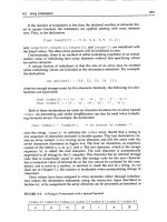
Since a simple process for taking square roots was known, Briggs computed

successive square roots of 10. A sample of the results is shown in Table 1.1.
The powers (x) of 10 are given in the first column and the results, 10
x
,are
given in the second column. For example, the second row is the square root
of 10, that is 10
1/2
=
√
10 = 3.16228. The third row is the square root of the
square root of 10,

10
1/2

1/2
=10
1/4
=1.77828. So on and so forth, we get a
series of successive square roots of 10. With a hand-held calculator, you can
readily verify these results.
In the table we noticed that when 10 is raised to a very small power, we
get 1 plus a small number. Furthermore, the small numbers that are added
16 1 Complex Numbers
Table 1.1. Successive square roots of ten
x (log N)10
x
(N)(10
x
− 1)/x

110.09.00
1
2
=0.53.16228 4.32
(
1
2
)
2
=0.25 1.77828 3.113
(
1
2
)
3
=0.125 1.33352 2.668
(
1
2
)
4
=0.0625 1.15478 2.476
(
1
2
)
5
=0.03125 1.074607 2.3874
(
1

2
)
6
=0.015625 1.036633 2.3445
(
1
2
)
7
=0.0078125 1.018152 2.3234
(
1
2
)
8
=0.00390625 1.0090350 2.3130
(
1
2
)
9
=0.001953125 1.0045073 2.3077
(
1
2
)
10
=0.00097656 1.0022511 2.3051
(
1

2
)
11
=0.00048828 1.0011249 2.3038
(
1
2
)
12
=0.00024414 1.0005623 2.3032
(
1
2
)
13
=0.00012207 1.000281117 2.3029
(
1
2
)
14
=0.000061035 1.000140548 2.3027
(
1
2
)
15
=0.0000305175 1.000070272 2.3027
(
1

2
)
16
=0.0000152587 1.000035135 2.3026
(
1
2
)
17
=0.0000076294 1.0000175675 2.3026
to 1 begins to look as though we are merely dividing by 2 each time we take
a square root. In other words, it looks that when x is very small, 10
x
− 1is
proportional to x. To find the proportionality constant, we list (10
x
− 1)/x
in column 3. At the top of the table, these ratios are not equal, but as they
come down, they get closer and closer to a constant value. To the accuracy of
five significant digits, the proportional constant is equal to 2.3026. So we find
that when s is very small
10
s
=1+2.3026s. (1.7)
Briggs computed successively 27 square roots of 10, and used (1.7) to obtain
another 27 squares roots.
Since 10
x
= N means x = log N, the first column in Table 1.1 is also the
logarithm of the corresponding number in the second column. For example,

the second row is the square root of 10, that is 10
1/2
=3.16228. Then by
definition, we know
log(3.16228) = 0.5.
If we want to know the logarithm of a particular number N, and N is not
exactly the same as one of the entries in the second column, we have to break
up N as a product of a series of numbers which are entries of the table. For
1.2 Logarithm 17
example, suppose we want to know the logarithm of 1.2. Here is what we do.
Let N =1.2, and we are going to find a series of n
i
in column 2 such that
N = n
1
n
2
n
3
··· .
Since all n
i
are greater than one, so n
i
<N. The number in column 2 closest
to 1.2 satisfying this condition is 1.15478, So we choose n
1
=1.15478, and we
have
N

n
1
=
1.2
1.15478
=1.039159 = n
2
n
3
··· .
The number smaller than and closest to 1.039159 is 1.036633. So we choose
n
2
=1.036633, thus
N
n
1
n
2
=
1.039159
1.036633
=1.0024367.
With n
3
=1.0022511, we have
N
n
1
n

2
n
3
=
1.0024367
1.0022511
=1.0001852.
The plan is to continue this way until the right-hand side is equal to one.
But most likely, sooner or later, the right-hand side will fall beyond the table
and is still not exactly equal to one. In our particular case, we can go down a
couple of more steps. But for the purpose of illustration, let us stop here. So
N = n
1
n
2
n
3
(1 + ∆n),
where ∆n =0.0001852. Now
log N = log n
1
+ log n
2
+ log n
3
+ log(1 + ∆n).
The terms on the right-hand side, except the last one, can be read from the
table. For the last term, we will make use of (1.7). By definition, if s is very
small, (1.7) can be written as
s = log(1 + 2.3026s).

Let ∆n =2.3026s, so s =
∆n
2.3026
=
0.0001852
2.3026
=8.04 ×10
−5
. It follows:
log(1 + ∆n) = log[1 + 2.3026

8.04 × 10
−5

]=8.04 ×10
−5
.
With log n
1
=0.0625, log n
2
=0.015625, log n
3
=0.0009765 from the table,
we arrived at
log(1.2) = 0.0625 + 0.015625 + 0.0009765 + 0.0000804 = 0.0791819.
The value of log(1.2) should be 0.0791812. Clearly if we have a larger table we
can have as many accurate digits as we want. In this way Briggs calculated the
logarithms to 16 decimal places and reduced them to 14 when he published his
table, so there were no rounding errors. With minor revisions, Briggs’ table

remained the basis for all subsequent logarithmic tables for the next 300 years.