Calculus: An Integrated Approach to Functions and their Rates of Change, Preliminary Edition Part 17 doc

4.1 Making Predictions: An Intuitive Approach to Local Linearity 141
change of −1 minute/day. Certainly it is ridiculous to estimate that on November 6, 1998,
the sun will set at 11:04 a.m. (where 5:09 p.m. −(1 minute/day)(365 days) = 5:09 p.m. −
365 minutes = 5:09 p.m. − (6 hours 5 minutes) = 11:04 a.m.)!
time
5:11
5:05
5:00
Nov. 410 25 2530 1515
Date (1997)
measured
by days
Dec.
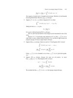
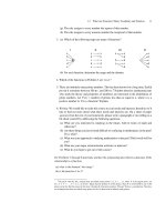
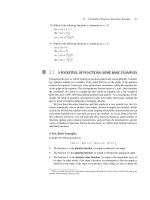
Sunset time Greenwich Mean Time at 30° North Latitude. time given to the nearest minute
Figure 4.2 Data from the 1998 World Almanac, pp. 463–474.
3
As we can see by looking at the graph in Figure 4.2, over small enough intervals, the
data points either lie on a line or lie close to some line that can be fitted to the data. However,
the line that fits the data best varies with the interval chosen. When looked at over the entire
interval from November 4 to December 25, the graph does not look linear.
◆
In the last example we looked at a discrete phenomenon and made predictions based
on the assumption of a constant rate of change over a small interval. In the next example
we’ll look at a continuous model.
◆
EXAMPLE 4.2 Brian Younger is a high-caliber distance swimmer; in competition he swam approximately
1 mile, 36 laps of a 25-yard pool.
4
If he completes the first 24 laps in 12 minutes, what
might you expect as his time for 36 laps?
SOLUTION Knowing that Brian is a distance swimmer, it is reasonable to assume that he does not

tire much in the last third. Assuming a constant speed of 12 laps every 6 minutes (or 120
yards/minute) we might expect him to finish 36 laps in about 18 minutes. We would feel
less confident saying that he could swim 4 miles if given an hour and 12 minutes, or 8 miles
if given 2 hours and 24 minutes.
◆
A quantity that changes at a constant rate increases or decreases linearly.
If the rate of change of height with respect to time,

 height
 time

,
is constant over a certain time interval, then height is a linear function of time on that
interval.
3
These times might look suspect to you; the sun begins to set later by December 10, well before the winter solstice. Do not
be alarmed: Sunrise gets later and later throughout December and continues this trend through the beginning of January.
4
One lap is 50 yards.
142 CHAPTER 4 Linearity and Local Linearity
If the rate of change of position with respect to time,

 position
 time

,
is constant, then position is a linear function of time.
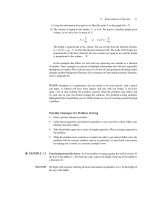
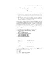
Think back to the bottle calibration problem. For a cylindrical beaker, the rate of change
of height with respect to volume is constant; height is a linear function of volume.
Cylindrical beaker

volume
height
Figure 4.3
Many of the functions that arise in everyday life (in fields like biology, environmental
science, physics, and economics) have the property of being locally linear. What does this
mean?
“Local” means “nearby” and “linear” means “like a line.”
5
So a function is locally linear
if, in the immediate neighborhood of any particular point on the graph, the graph “looks like
a line.” This is not to say that the function is linear; we mean that near a particular point the
function can be well approximated by a line. In other words, over a small enough interval,
the rate of change of the function is approximately constant.
Graphically this means that f is locally linear at a point A if, when the graph is
sufficiently magnified around point A, the graph looks like a straight line.
6
The questions
of which line best approximates the function at a particular point and just what we mean by
“nearby” are very important ones, and we will examine them more closely in chapters to
come. First, let’s look back at Examples 4.1 and 4.2.
In Example 4.1 the runner estimating the time of sunset is assuming local linearity;
her assumption leads to a prediction that is only 1 minute off when she predicts just a few
days ahead. The function is only locally linear; the idea of “locality” does not extend from
the first three readings in early November all the way to Christmas day. In Example 4.2 the
assumption that the swimmer’s pace is maintained for another 5 minutes is an assumption
of local linearity.
You probably have made many predictions of your own based on the assumption of
local linearity without explicitly thinking about it. For instance, if you buy a gallon of milk
and you have only a quarter of a gallon left after three days, you might figure that you’ll be
out of milk in another day. Here you’re assuming that you will consume milk at a constant

rate of
1
4
gallon/day. Or, suppose you come down with a sore throat one evening and take
three throat lozenges in four hours. You might take six lozenges to work with you the next
day, assuming that you’ll continue to use them at a rate of
3
4
lozenge/hour for eight hours.
5
By “line” we mean straight line.
6
A computer or graphing calculator can help you get a feel for this if you “zoom in” on point A.
4.2 Linear Functions 143
Clearly you wouldn’t expect to pack six lozenges with you every day; you’re assuming only
local linearity.
Many examples of the use of local linearity arise in the fields of finance and economics.
Investors lay billions of dollars on the line when they use economic data to project into the
future. The question of exactly how far into the future one can, within reason, linearly project
any economic function based on its current rate of change, and by how much this projection
may be inaccurate, is a matter of intense discussion.
Local linearity plays a key role in calculus. The problem of finding the best linear
approximation to a function at a given point is a problem at the heart of calculus. In order
to work on this keystone problem, one must be very comfortable with linear functions. So,
before going on, let’s discuss them.
PROBLEMS FOR SECTION 4.1
1. Lucia has decided to take up swimming. She begins her self-designed swimming
program by swimming 20 lengths of a 25-yard pool. Every 4 days she adds 2 lengths
to her workout. Model this situation using a continuous function. In what way is this
model not a completely accurate reflection of reality?

2. Cindy quit her job as a manager in Chicago’s corporate world, put on a backpack,
and is now traveling around the globe. Upon arrival in Cairo, she spent $34 the first
day, including the cost of an Egyptian visa. Over the course of the next four days, she
spent a total of $72 on food, lodging, transportation, museum entry fees, and baksheesh
(tips). She is going to the bank to change enough money to last for three more days in
Cairo. How much money might she estimate she’ll need? Upon what assumptions is
this estimate based?
3. It is 10:30 a.m. Over the past half hour six customers have walked into the corner
delicatessen. How many people might the owner expect to miss if he were to close the
deli to run an errand for the next 15 minutes? Upon what assumption is this based?
Suppose that between 9:30 a.m. and 11:30 a.m. he had 24 customers. Is it reason-
able to assume that between 11:30 a.m. and 1:30 p.m. he will have 24 more customers?
Why or why not?
4.2 LINEAR FUNCTIONS
The defining characteristic of a linear function is its constant rate of change.
◆
EXAMPLE 4.3 For each situation described below, write a function modeling the situation. What is the rate
of change of the function?
(a) A salesman gets a base salary of $250 per week plus an additional $10 commission for
every item he sells. Let S(x) be his weekly salary in dollars, where x is the number of
items he sells during the week.
144 CHAPTER 4 Linearity and Local Linearity
(b) A woman is traveling west on the Massachusetts Turnpike, maintaining a speed of 60
miles per hour for several hours. Her odometer reads 4280 miles when she passes the
Allston/Brighton exit. Let D(t) be her odometer reading t hours later.
SOLUTION (a)
salary = base salary + commission
salary = base salary +

dollars

item

(items)
S(x) = 250 + 10x
The rate of change of S =
S
x
= $10 per item.
(b)
odometer reading = (initial odometer reading) + (additional distance traveled)
odometer reading = (initial reading) +

miles
hour

(hours)
D(t) = 4280 + 60t
The rate of change of D =
D
t
= 60 miles per hour.
◆
Definition
f is a linear function of x if f can be written in the form f(x)=mx + b, where m
and b are constants.
The graph of a linear function of one variable is a straight nonvertical line; conversely,
any straight nonvertical line is the graph of a linear function. As we will show, the line
y = mx + b has slope m and y-intercept b. The slope corresponds to the rate of change
of y with respect to x. Every point (x
0

, y
0
) that lies on the graph of the line satisfies the
equation. In other words, if (x
0
, y
0
) lies on the graph of y = mx + b, then y
0
= mx
0
+ b.
Conversely, every point whose coordinates satisfy the equation of the line lies on the graph
of the equation. As discussed in Chapter 1, this is what it means to be the graph of a function.
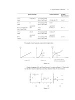
The following are examples of equations of lines and their graphs.
1
–1
1
2
f
x
Figure 4.4 f(x)=2x−1
m=2, b =−1
4.2 Linear Functions 145
f
x
Figure 4.5 f(x)=
√
10
m = 0, b =

√
10
–2 –112
1
1
f
x
Figure 4.6 f(x)=−0.5x
m =−0.5, b =0
The slope of a line is the ratio
rise
run
,or
change in dependent variable
change in independent variable
.
If y is a linear function of x, then the slope is
change in y
change in x
,or
y
x
.
We will now verify that if y = mx + b, then the constant m is the slope of the line.
Verification: Suppose (x
1
, y
1
) and (x
2

, y
2
) are two distinct points on the graph of
y = mx + b. We want to show that the rate of change of y with respect to x is m, regardless
of our choice of points.
Since y = mx + b, the points (x
1
, y
1
) and (x
2
, y
2
) can be written as (x
1
, mx
1
+ b) and
(x
2
, mx
2
+ b).
146 CHAPTER 4 Linearity and Local Linearity
∆y
∆ x
(x
2
, y
2

) = (x
2
, mx
2
+ b)
(x
1
, y
1
) = (x
1
, mx
1
+ b)
Figure 4.7
Therefore,
change in y
change in x
=
y
x
=
y
2
− y
1
x
2
− x
1

=
(mx
2
+ b) − (mx
1
+ b)
x
2
− x
1
=
mx
2
− mx
1
x
2
− x
1
=
m(x
2
− x
1
)
x
2
− x
1
= m

We have shown that the slope of the line y = mx + b is indeed m. The slope of a line
is a fixed constant, regardless of how it is computed.
To verify that b is the y-intercept of the line, we set x = 0. Then y = m · 0 + b = b.
(Remember that the y-intercept is the value of the function on the y-axis, i.e., when x = 0.)
◆
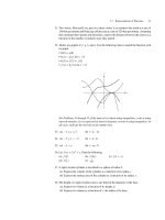
EXAMPLE 4.4 3x + 2y = 7 is the equation of a line. Find the slope and the x- and y-intercepts.
SOLUTION Put the equation into the form y =−
3
2
x +
7
2
. We can then read off the y-intercept as
7
2
and the slope as −
3
2
.
Find the x-intercept by setting y = 0:
3x + 2(0) = 7
3x = 7
x =
7
3
.
Alternatively, begin with 3x + 2y = 7 and find the x-intercept by setting y = 0 and
solving for x: (
7
3

,0).Find the y-intercept by setting x = 0 and solving for y: (0,
7
2
).
(The x- and y-intercepts can be useful in graphing the line.) Given any two points, you
can find the slope by computing
y
x
. For instance, given the points (
7
3
,0)and (0,
7
2
),
the slope is computed as follows.
y
x
=
7
2
− 0
0 −
7
3
=
7
2
−
7

3
=

7
2

−
3
7

=−
3
2
4.2 Linear Functions 147
y
x
1
12
3
4
–1
–2
2
3
5
7
2
7
3
Figure 4.8

It is not necessary to use the x- and y-intercepts in order to calculate the slope; any two
points will do.
◆
EXERCISE 4.1 Verify that any equation of the form ax + cy = d, where a, c, and d are constants and c = 0
is a linear equation. In other words, verify that it can be written in the form y = mx + b.If
ax + cy = d, what is
y
x
?
Lines and Linear Equations
EXERCISE 4.2 Graph the following lines. Use three sets of axes, one for each of the Parts I, II, and III.
I. a) y = x b) y = 2x c) y = 3x d) y = 0.5x e) y =−2x f) y =−0.5x
II. a) y = 2x b) y = 2x + 1c)y=2x−2
III. a) y = 3b)x=4c)x=0d)y=0
Notice that the results of this exercise are consistent with the principles of stretching,
shrinking, flipping, and shifting discussed in Section 3.4.
From this exercise you can observe how the constant m corresponds to the steepness
of the line.
m = 0 ⇒ The line is horizontal.
m>0 ⇒ The line rises from left to right, so the function is increasing.
The more positive m is, the steeper the rise of the line.
m<0 ⇒ The line falls from left to right, so the function is decreasing.
The more negative m is, the steeper the fall of the line.
The closer m is to zero, the less steep the line.
Vertical Lines
A vertical line is the graph of an equation of the form x = constant. Notice that a vertical
line is not the graph of a function of x. One x-value is mapped to infinitely many y-values;
a vertical line certainly fails the vertical line test!
148 CHAPTER 4 Linearity and Local Linearity
x=3

x
yy
slope undefined
x
y=1
slope = 0
Figure 4.9
Slope =
y
x
, so the slope of a vertical line is undefined, while the slope of a horizontal line
is zero.
Parallel and Perpendicular Lines
If L
1
and L
2
are nonvertical lines with slopes m
1
and m
2
, respectively, then
L
1
is parallel to L
2
if and only if m
1
= m
2

, i.e., their slopes are equal.
L
1
is perpendicular to L
2
if and only if m
1
=
−1
m
2
, i.e., their slopes are negative
reciprocals.
Fundamental Observation
A line is completely determined by either
i. the slope of the line and any one point on the line, or
ii. any two points on the line.
This geometric observation can be translated as follows. If there is a linear relationship
between two variables, then that relationship can be completely determined provided
i. one data point is known and the rate of change of one variable with respect to the other
is known, or
ii. two data points are known.
Finding the Equation of a Line
i. Suppose we know the slope of the line, m, and a point on the line, (x
1
, y
1
).Wecanfind
the equation of the line by using either of the following two methods.
.

Method 1: The equation of any nonvertical line can be put into the form y = mx + b.
If we know the slope, we know m. Our job is to find b. Because (x
1
, y
1
) is a point on
the line, (x
1
, y
1
) satisfies the equation y = mx + b. Therefore, y
1
= mx
1
+ b, where
x
1
, y
1
, and m are constants. We can solve for b, the only unknown, and then write
y = mx + b.
.
Method 2: The slope =
y
x
. Point (x
1
, y
1
) is a fixed point on the line. Therefore, if

(x, y) lies on the line,
m =
y − y
1
x − x
1
.
This is written
y − y
1
= m(x − x
1
)
4.2 Linear Functions 149
to make it clear that the domain is all real numbers. Solving for y will put this into
the form y = mx + b.
The equation y − y
1
= m(x − x
1
) is called the point-slope form of the equation
of a line.
ii. Suppose we know two points on a line: (x
1
, y
1
) and (x
2
, y
2

).Wecanfind the slope of
the line:
y
x
=
y
2
− y
1
x
2
− x
1
= m.
Knowing the slope and a point (two points, actually), we can continue as described in
part i.
◆
EXAMPLE 4.5 Find the equation of the line passing through points (2, −3) and (−4, 5).
SOLUTION Calculate the slope.
m =
−3 − 5
2 − (−4)
=
−8
6
=−
4
3
,
so

y =−
4
3
x + b.
Use the fact that point (2, −3) lies on the line to find b.
−3 =−
4
3
(2) + b ⇒ b =−3+
8
3
=−
9
3
+
8
3
=−
1
3
y =−
4
3
x −
1
3
.
Alternatively, after finding m =−
4
3

we can use Method 2 above.
−
4
3
=
y + 3
x − 2
y + 3 =−
4
3
(x − 2)
We leave it up to you to verify that the equations are equivalent.
◆
The Equation of a Line
Slope-intercept form of a line Point-slope form of a line
y = mx + by−y
1
=m(x − x
1
)
where m is the slope and b is the y-intercept where m is the slope and (x
1
, y
1
) is a point
on the line
150 CHAPTER 4 Linearity and Local Linearity
Scientists and social scientists often make general models in which constants or pa-
rameters are represented by letters.
7

Cases in which the slope and/or points of a line are not
given as numbers but as letters representing constants typically are stumbling blocks for
students trying to determine the equation of the line. Unless you think carefully and clearly,
it is easy to lose track of the main features of the equation:
the two variables,
the constants that are given, and
the unknown constants that you are trying to find.
If you plan to consider slope, you must decide which variable will play the role of the inde-
pendent variable and which will be treated as the dependent variable. (If you’re accustomed
to x’s and y’s, then determine which variable will play the role of x and which will play the
role of y.) By taking inventory, keeping your goal firmly in mind, and determining the steps
you’ll take to reach that goal, you ought to be able to proceed fearlessly. Try the following
exercises.
EXERCISE 4.3
i. Find the equation of the line through the points (2π, π
2
) and

π,
1
π

.
ii. Find the equation of the line through the point (a, c
2
) having slope p.
iii. Find the equation of the line through (m, n) with slope b.
CAUTION Here m and b are playing nonstandard roles. To avoid confusion, try a strategic
maneuver; use something such as y = Ax + C as your “reference” equation to avoid getting
the m’s and b’s in the problem confused with the slope and the y-intercept.)

EXERCISE 4.4 Over the interval [0, T ] a horse’s velocity, v, is a linear function of time, t .
(a) At time t = 0, the horse’s velocity is v
0
. At time t = T, his velocity is v
T
. Find v(t) on
the interval [0, T ]. Note: v
0
, T, and v
T
are all constants.
(b) What can you say about the horse’s acceleration?
Answers to Selected Exercises
Answers to Exercise 4.3
i. y =
π
3
−1
π
2
x − π
2
+
2
π
ii. y = px + c
2
− pa
iii. y = bx + n − mb
Answers to Exercise 4.4:

(a) v(t) = mt + b because v is a linear function of t. Our job is to find m and b.Weare
given two points, (0, v
0
) and (T, v
T
). (Points are written in the form (time, velocity)
because time is the independent variable.) In other words, t plays the role of x and v
7
Physicists use g to denote acceleration due to the force of gravity. Biologists might denote the carrying capacity of an ecosytem
for a certain species by a letter, such as C, without specifying the value of C. Chemists use r for Avogadro’s number, the number
of molecules in a mole.