Financial Modeling with Crystal Ball and Excel Chapter 5 pot

CHAPTER
5
Using Decision Variables
T
he first four chapters covered the basics of specifying Crystal Ball assumptions
and analyzing Crystal Ball forecasts. This chapter covers the basics of defining
and using Crystal Ball decision variables and its decision support tools, Decision
Table and OptQuest.
DEFINING DECISION VARIABLES
Decision variables are spreadsheet cells in which the values are varied systemat-
ically rather than sampled randomly, as are assumptions. They can be cells that
hold values dictated by actual decisions or cells for which we just want to see
the effect of one or two variables on selected forecasts in a form of sensitivity
analysis.
As an example of the latter, consider the model depicted in Figure 5.1,
TwoCorrelatedAssets.xls, where we have two correlated assets and we wish to
vary the correlation coefficient to see the effect on the rate of return of a portfolio
composed of the two assets. To keep things simple we will simulate a model for
which we know the true answer so that we can compare the simulation results to
the truth.
Consider a portfolio composed of two assets, A and B. Asset A has a normally
distributed rate of return with mean, µ
A
= 10 percent, and standard deviation,
σ
A
= 20 percent. Asset B has a normally distributed rate of return with mean,
µ
A
= 15 percent, and standard deviation, σ
B

= 30 percent. We will invest half of
our available funds in Asset A and half in Asset B, and we are interested in seeing
how the distribution of the rate of return of our portfolio varies as a function of
the correlation coefficient, ρ, between the rates of return on Assets A and B. In
Two Correlated Assets.xls, cells A9 and A10 are assumptions, and cell A13 is a
forecast.
The assumptions in cells A9 and A10 of the file TwoCorrelatedAssets.xls are
defined as normal distributions as described in Chapter 4. However, to reflect the
limited liability of stock ownership, the rates of return on both assets are truncated
71
72 FINANCIAL MODELING WITH CRYSTAL BALL AND EXCEL
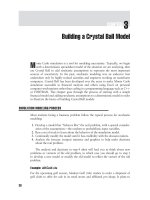
FIGURE 5.1 Spreadsheet model in
file TwoCorrelatedAssets.xls, which models rate
of return on portfolio as the correlation
coefficient, ρ, varies from −1.00 to +1.00 in
steps of 0.25. Cell D5 is a decision variable,
cells A9 and A10 are assumptions, and cell A13 is
a forecast.
on the left at −100 percent. This is accomplished by entering this value in the
field directly above the Mean field as shown in Figure 5.2 for the rate of return
assumption for Asset B. With a mean of 15 percent and a standard deviation of
30 percent, the normal distribution will rarely produce any values below −100%
(which is more than 3.8 standard deviations below the mean), but truncating the
distribution ensures that on those rare occasions when a value less than −100%
is generated from a nontruncated normal distribution for Asset B, Crystal Ball will
discard it and generate another random value in its place. Asset A’s rate of return is
also bounded from below by −100%.
Note that the title bar of the dialog in Figure 5.2 for cell A10 indicates that it is
correlated with another assumption, in this case the assumption in cell A9.During
any simulation run, the correlation coefficient is the value in cell D5,whichiswhat

we will vary with the Decision Table tool.
To make Cell D5 into a decision variable, first click on it. Then select
Define→Define Decision from the top menu or click on the Define Decision
icon on the Crystal Ball toolbar. Fill in the fields as shown in Figure 5.3. This
tells Crystal Ball that you wish to vary the value in cell D5 from −1.00 to +1.00
in discrete steps of 0.25. Click OK and cell D5’s background will turn yellow to
indicate that a decision variable is defined in that cell. You are now ready to use the
Decision Table tool or OptQuest with the model.
Using Decision Variables
73
FIGURE 5.2 Define assumption dialog for cell A10 in
file TwoCorrelatedAssets.xls.
FIGURE 5.3 Define Decision Variable dialog window.
DECISION TABLE WITH ONE DECISION VARIABLE
Select Run→Tools→Decision Table from the top menu. You will get a dialog
window for step 1 like that shown in Figure 5.4. For models with more than one
forecast defined, you would first highlight the forecast for which you wish to
analyze the sensitivity to the decision variable. As there is only one forecast in this
model, there is no choice to be made here, so click Next > to select the forecast
Portfolio ROR.
74 FINANCIAL MODELING WITH CRYSTAL BALL AND EXCEL
FIGURE 5.4 Dialog window for step 1 of using Decision Table.
The dialog for step 2 is where you choose the decision variables to evaluate,
as shown in Figure 5.5. Again, because there is only one decision variable defined,
click >> to move the decision variable Correlation to the Chosen Decision Variables
field, then click Next>.
Step 3 is where you specify the Decision Table options. Take the default options
depicted in Figure 5.6, then click Start. Crystal Ball will begin running nine sets of
10,000 simulation trials, one set for each of the following values of the correlation
coefficient:

{−1.00, −0.75, −0.50, −0.25, 0.00, 0.25, 0.50, 0.75, 1.00}
After it has finished running 90,000 simulation trials, Crystal Ball will create
a separate workbook like that in Figure 5.7 holding nine forecasts and three
buttons:Trend Chart, Overlay Chart,andForecast Charts.
Trend Chart
To see the trend chart, select the forecasts in cells B2:J2, then click Trend Chart
to get a graphical display similar that shown in Figure 5.8. A trend chart displays
the certainty bands for several forecasts on one plot. The chart in Figure 5.8 clearly
Using Decision Variables
75
FIGURE 5.5 Dialog window for step 2 of using Decision Table.
FIGURE 5.6 Dialog window for step 3 of using Decision Table.
76 FINANCIAL MODELING WITH CRYSTAL BALL AND EXCEL
FIGURE 5.7 Results of using Decision Table.
FIGURE 5.8 Trend chart displaying results of using Decision Table.
shows how the variability of the portfolio rate of return increases as the correlation
coefficient goes from −1.00 to +1.00. At the left end of the trend chart, the 90
percent certainty band extends from 4.3 percent to 20.7 percent for the forecast
Portfolio ROR (1), which is the forecast generated when the correlation coefficient is
−1.00. At the right end, the 90 percent certainty band extends from −28.6 percent
to 53.6 percent for the forecast Portfolio ROR (9), which is the forecast generated
when the correlation coefficient is +1.00. These correspond to the same certainty
intervals indicated in the forecast charts for Portfolio ROR (1) and Portfolio ROR (9)
displayed in Figure 5.9.
Note how the certainty bands diverge from left to right, but remain centered
on 12.5 percent. They correspond very well to the theoretical bounds calculated in
Two Correlated Assets.xls, and displayed in Figure 5.10.
Using Decision Variables
77
FIGURE 5.9 Frequency charts for Portfolio ROR (1) and (9) from

Decision Table results.
These charts conform well to theory, which holds that the rate of return on
the portfolio will be normally distributed with mean µ
P
= wµ
A
+(1 −w)σ
B
,and
standard deviation
σ
P
=

w
2
σ
2
A
+(1 −w)
2
σ
2
B
+2w(1 − w)ρσ
A
σ
B
, (5.1)
where w is the weight (0 ≤ w ≤ 1) of Asset A in the portfolio. For this example,

w = 0.5.
78 FINANCIAL MODELING WITH CRYSTAL BALL AND EXCEL
FIGURE 5.10 Theoretical 90 percent certainty
bounds for trend chart displaying results of using
Decision Table. Bounds are calculated as
µ
P
+
−1
(y)σ
P
,where
−1
(y) is the inverse CDF for
the standard normal distribution, y = 0.05 for the
lower bound, and y = 0.95 for the upper bound.
It is worth noting that our model differed slightly in at least two ways from
the theoretical model underlying Expression (5.1). First, Crystal Ball uses Spear-
man correlation, ρ
S
, for sampling instead of the Pearson correlation, ρ,usedin
Expression (5.1); however, for normally distributed rates of return this makes little
difference. Second, we truncated the rate of return assumptions on the left, which
has the effect of changing the standard deviations slightly, but this also made little
difference.
Overlay Chart
The forecast charts in Figure 5.9 look similar, but the scales of their horizontal axes
are much different. To make it easier to compare forecasts, use an overlay chart. Click
on cell B2, then hold down the Ctrl key and click on cell J2 to select the forecasts
Using Decision Variables

79
FIGURE 5.11 Overlay chart displaying results of using Decision
Table.
for Portfolio ROR (1) and Portfolio ROR (9).ThenclicktheOverlay Chart button to
get a chart like that displayed in Figure 5.11, which clearly shows the difference in
dispersion between the forecasts for Portfolio ROR (1) and Portfolio ROR (9).You
can create an overlay chart for more than two forecasts at a time, but do so with
care as they become hard to read when too many forecasts are included.
DECISION TABLE WITH TWO DECISION VARIABLES
You can also use the Decision Table tool with two decision variables. The output is
similar to the output with one decision variable, except that Crystal Ball will produce
an array containing a forecast for every possible combination of the values specified
for each decision. This section contains an example of using Decision Table with a
model built as an illustration of how to estimate a value for managerial flexibility.
Model
For an example of a situation with two decision variables, suppose that a firm can
invest in a project having a three-year life and a terminal value that depends on the
cash flow in the final quarter of the third year. Suppose further that there are only
two sources of uncertainty: (1) the average quarterly growth rate of revenue, and (2)
variable cost as a percentage of revenue. We assume that average quarterly revenue
growth is random and follows a normal distribution with mean = 5 percent, and
standard deviation = 5 percent. Variable cost as a percentage of revenue is also
80 FINANCIAL MODELING WITH CRYSTAL BALL AND EXCEL
FIGURE 5.12 Spreadsheet segment from Project.xls. Note that columns E through K are hidden.
normally distributed with a mean of 50 percent, and a standard deviation of 5
percent. The discount rate is assumed to be 12.5 percent. Figure 5.12 shows a
spreadsheet segment from Project.xls that is used to value this project with net
present value (NPV). For the purposes of this example, we will use the Mean of the
NPV forecast, ENPV, as the value of the project.
By looking at this project from different perspectives, we can estimate the value

of the project manager’s flexibility over time to affect the course of the project. To
estimate the value of this flexibility, we consider two scenarios to find:
ENPV 1 = The value of the project without managerial flexibility; and
ENPV 2 = The value of the project with managerial flexibility.
The value of the managerial flexibility is then determined as the difference between
ENPV 1 and ENPV 2.
With a standard NPV analysis, we assume that the project manager has no
flexibility to make decisions during the life of the project. That is, once the project
Using Decision Variables
81
is begun it is run to the end of three years with no expansion if successful, and no
abandonment if unsuccessful.
Open the file Project.xls and run the simulation model. When the simulation
stops, look at the Crystal Ball forecast window for NPV 1, which is also shown in
Figure 5.13. The mean net present value is $18.61, which is the value of the project
with no flexibility. Note that the output in Figure 5.13 also shows the probability is
only about 40 percent that the project will add value to the firm, because the value
in the certainty field at the bottom center of the forecast window is 42.92 percent.
Now suppose that we are faced with a similar situation, but this time we have
the option to abandon the project if unfavorable circumstances occur. For now,
let’s use the following decision rule for abandonment. Begin checking in the second
quarter of Year 2, and abandon the project if three consecutive quarters of negative
cash flow occur. This decision rule is built into rows 50 and 51 of Project.xls with
indicator variables, as shown in Figure 5.14. Cells G50:M50 check whether or not to
abandon each quarter, and cells G51:M51 ensure that once abandoned, the project
contributes no positive cash flows in future quarters.
The Crystal Ball output in Figure 5.15 shows that the option to abandon has
increased the project’s value. Because the mean NPV with abandonment possible is
$50.62, the value of the abandonment option is estimated to be $50.62 − $18.61
= $32.01. Note that the flexibility to abandon the project does not change the

inherent risk structure of the project itself, so in Figure 5.15 the probability that the
project adds value to the firm remains the same, that is, Pr(NPV > 0) ≈ 40 percent.
FIGURE 5.13 Crystal Ball forecast for NPV1 for the case of no flexibility
in the Project.xls model.
82 FINANCIAL MODELING WITH CRYSTAL BALL AND EXCEL
FIGURE 5.14 Spreadsheet segment from Project.xls model showing the possibility
of abandonment. Note that columns E through K are hidden.
FIGURE 5.15 CB forecast window from Project.xls model showing the
possibility of abandonment.
Using Decision Variables
83
However, by allowing for abandonment, we limit the losses incurred by the firm,
just as an active and astute project manager would do in a real-world situation.
Because of the ability to limit losses in the left tail of the distribution, the manager’s
flexibility increases the ENPV of the project.
Now consider another option the manager has with this project, the option to
expand if favorable conditions occur. To value the expansion option, we use the
following decision rule. Begin checking in the second quarter of Year 2, and expand
if we see three consecutive quarters of cash flow greater than $15. The investment
in the expansion project will cost $200, and we assume that expansion will double
the quarterly revenue and expenses. This decision rule is built into rows 77 and 78
of the spreadsheet model in Project.xls shown in Figure 5.16.
FIGURE 5.16 Spreadsheet segment from Project.xls model showing the possibilities of abandonment
and expansion. Note that columns E through K are hidden.
84 FINANCIAL MODELING WITH CRYSTAL BALL AND EXCEL
FIGURE 5.17 CB forecast window from Project.xls model showing
the possibility of expansion.
The Crystal Ball output in Figure 5.17 shows that the option to expand the
project has vastly increased its value. Because the mean NPV with both expansion
and abandonment possible is $290.03, the value of the expansion option is $290.03

− $50.62 = $239.41. Note that the flexibility to expand the project did change its
inherent risk structure slightly, in that the the probability that the project adds value
to the firm increased a bit, that is Pr(NPV > 0) ≈ 48 percent. If you extract the
data, you will see that on about 500 trials, the value of NPV 3 was positive while
NPV 2 was negative. In this situation we model the realistic behavior of an active
decision maker who will capitalize on fortuitous conditions that promote expansion.
By expanding when times are good, the decision maker increases the ENPV of the
project by adding gains to the right tail of the distribution of possible results.
Threshold Values
In the previous example we arbitrarily specified the decision rule for project aban-
donment as ‘‘abandon the project if three consecutive quarters of negative cash flow
occur.’’ Likewise, we arbitrarily specified the decision rule for project expansion as
‘‘expand if we see three consecutive quarters of cash flow greater than $15.’’ By
adding decision variables to the model we can use the Decision Table tool to help
determine if the arbitrary threshold dollar amounts of $0 for abandonment and
$15 for expansion are the optimal values to use. That is to say, it is possible that
some other threshold values, such as −$5 and $20 might yield higher option values
and if so we would like to find the threshold values that yield the highest option
values. Note that we could also use decision variables to determine whether using
Using Decision Variables
85
FIGURE 5.18 Decision variables for the threshold value at which to
abandon and expand in the Project.xls model.
two or four (or some other number) of consecutive quarters is optimal; however, for
illustrative purposes here we will stick to threshold dollar amounts of cash flow.
To see the decision variable for the threshold value of cash flow for aban-
doning the project, click on cell B4 in Project.xls. Then click on Define→Define
Decision on the top menu in Excel. This will bring up the dialog window shown
at the top of Figure 5.18. Cell B4 is named ‘‘Abandon Point,’’ and Crystal Ball will
consider four different values, {0, −3, −6, −9}. Note that we specified discrete steps

of $3, but by clicking the Continuous button in the Variable Type section of the
dialog window, we could have had Crystal Ball investigate the potentially infinite
number of values between virtually any specified lower and upper bounds. Using a
discrete variable type limits the number of values that Crystal Ball checks and thus
speeds up the analysis.
86 FINANCIAL MODELING WITH CRYSTAL BALL AND EXCEL
To see the decision variable for threshold value of cash flow for expanding the
project, click on cell B5 in Project.xls.ThenclickonDefine→Define Decision on
the top menu in Excel. This will bring up the dialog window shown at the bottom
of Figure 5.18. We have named this decision variable ‘‘Expansion Point’’ and have
told Crystal Ball to consider seven different values, {0, 5, 10, ,30}. Note that we
specified discrete steps of $5 here to speed up the analysis and simplify the results
displayed in the next section.
Two-Way Decision Table
With the decision variables for cells B4 and B5 as defined in the previous section, we
can use Crystal Ball’s decision table tool to find the optimal combination of values
for Abandon Point and Expansion Point.
1. In the top menu, click on Run→Tools→Decision Table tobringupStep1of
the Decision Table tool (see Figure 5.19). Select the target forecast NPV 3 as
shown in Figure 5.19). Click the Next> button to continue.
FIGURE 5.19 Step 1 in using the Decision Table tool with the Project.xls model.
Using Decision Variables
87
FIGURE 5.20 Step 2 in using the Decision Table tool with the Project.xls model.
2. Use the >> button to move the decision variables Abandon Point and Expansion
Point into the Chosen Decision Variables box on the right side of the dialog box
as shown in Figure 5.20. Click the Next> button to continue.
3. Take the default values for the fields in the step 3 dialog box as shown in
Figure 5.21. Click the Start button to tell Crystal Ball to use the decision table
tool to evaluate all possible combinations of the specified values of Abandon

Point and Expansion Point.
You have just instructed Crystal Ball to run 10,000 trials for each of 4 × 7 = 28
different combinations of decision variable values. The amount of time it takes
Crystal Ball to run these 280,000 iterations depends on the speed of your computer.
Interpreting the Results
Figure 5.22 shows the results of using the decision table tool. Cell C3 contains
the maximum expected NPV of $299.78, which results from using the following
decision rules: (1) Begin checking in the second quarter of year, and abandon the
project if three consecutive quarters of cash flow below −$6 occur; and (2) expand if
88 FINANCIAL MODELING WITH CRYSTAL BALL AND EXCEL
FIGURE 5.21 Step 3 in using the Decision Table tool with the Project.xls model.
FIGURE 5.22 Results from using the Decision Table tool with the
Project.xls model.
Using Decision Variables
89
three consecutive quarters of cash flow greater than $5 occur. These new threshold
values of −6 and 5 are shown in the labels occupying cells C1 and A3, respectively,
in Figure 5.22. Note that the maximum value of $299.78 identified in the Decision
Table tool output is $9.75 greater than the $290.03 identified in Figure 5.17. Keep
in mind, though, that these figures are just estimates based on 10,000 runs of the
simulation. More runs would result in higher precision of the estimates.
At its heart, Monte Carlo simulation is just a computer-based sampling system.
Thus, specifying more runs of the simulation will yield more precise results just as
including more items in a random sample yields more precise estimates in a statistical
study designed to make inferences about a population. Crystal Ball allows you to
specify the level of precision that you desire. See Chapter 6 for information on how
to specify the precision level.
In this example, we varied the Abandon Point in steps of $3, and the expansion
Point in steps of $5. We might be able to identify even higher levels of expected NPV
by using smaller steps.

The Decision Table tool works well to find the optimal solution for problems
involving one or two decision variables. It also serves to introduce the notion of
simulation optimization, which is the process of finding the best values of decision
variables that we just completed for abandon point and expansion point. When more
than two decision variables are involved, as is typical for more realistic problems,
the add-in OptQuest is a more powerful tool for finding an optimal solution. This
is the topic of the next section.
USING OPTQUEST
We saw in the last section how a decision table could be set up to find the value
of a designated output for selected combinations of two decision variable values.
Once that was accomplished, we found the best solution by looking at the values
in the table to locate the combination that gave the maximum value of the output.
Decision tables work very well for one or two decision variables. However, if there
are more than two decision variables, decision tables are cumbersome. This section
describes how to use the Crystal Ball tool OptQuest to help find the best decisions
to make in situations involving more than two decisions.
Terminology
In order to understand better how OptQuest works, some background knowledge of
the terminology is required. This subsection gives definitions for some of the terms
that will be used throughout the rest of this section.
Constraint. A constraint is a relationship among decision variables that
restricts the values of the decision variables. When you define a decision
variable, you constrain it individually by specifying the bounds. However,
90 FINANCIAL MODELING WITH CRYSTAL BALL AND EXCEL
TABLE 5.1 Forecast statistics available for optimizing or using in a
requirement with OptQuest.
Mean Percentile Mean standard error
Median Skewness Certainty
Mode Kurtosis Final value
Standard deviation Coefficient of variability

Variance Range
with an OptQuest constraint, you can restrict the values of linear combina-
tions of decision variables. For example, an OptQuest constraint might be
used to ensure that the sum of weights in a portfolio of assets is equal to
1.0.
Objective. An objective gives a mathematical representation of the criterion
by which it will be determined what is best or optimal. For the Project.xls
model, the objective is the maximization of mean net present value (ENPV)
because NPV is a direct measure of the value added to the firm by actions
undertaken by a decision maker. However, other objectives could also be
chosen, such as minimizing the cost or the riskiness of a decision.
Forecast statistic. A forecast statistic is a summary value of a forecast distribu-
tion, such as the mean, standard deviation, or variance. The optimization
is controlled by maximizing, minimizing, or restricting a selected forecast
statistic. For example, in the Project.xls model, we chose to maximize the
mean NPV because doing so will, on average, give the best results. Thus,
maximizing the mean of a forecast is a good strategy for a firm that makes
many decisions on a periodic basis. An individual or a firm that is more
risk-averse, however, might choose to minimize the standard deviation,
or maximize the 5th percentile of the forecast distribution, for example.
Table 5.1 lists the forecast statistics available for optimizing or using in a
requirement.
Requirement. A requirement is a restriction on a forecast statistic that you
can set while trying to optimize on some other statistic. For example,
you might be interested in maximizing the mean return on a retirement
portfolio while at the same time requiring that the risk as measured by
the standard deviation does not exceed some specified value. You can use
requirements to set upper and lower limits for any statistic of a forecast
distribution.
Example

Open Project.xls,thengotothetopmenuandselectRun→OptQuest. In OptQuest,
select File→New. This will start a wizard that will lead you through the dialog
windows to set up the tool. The Decision Variable Selection window appears first,
Using Decision Variables
91
FIGURE 5.23 Decision Variable Selection window for the Project.xls model.
FIGURE 5.24 Constraints window for the
Project.xls model.
listing every decision variable defined in the Crystal Ball model. Your window should
look like the one shown in Figure 5.23.
The window in Figure 5.23 lets you select which defined decision variables to
optimize. The columns and buttons are mostly self-explanatory, although it might
not be immediately apparent that Suggested Value is simply the value that is in the
decision variable cell when OptQuest is started. To follow this example, you need
only to use the default values, so click OK to continue.
The next window that appears is the Constraints window, which is shown in
Figure 5.24.
In OptQuest, constraints limit the possible solutions to a model in terms of
relationships among the decision variables. In Version 2.3 of OptQuest, you can use
the Constraints window to specify only linear constraints. In the Project.xls model,
we have no constraints on the decision variables (except for the bounds, which we
specify when defining the decision variables), so click on OK to continue.
After you exit the Constraints window, the Forecast Selection window appears
next, listing all the forecasts defined in the model as shown in Figure 5.25. In the
forecast row for NPV 3,clickintheSelect column. From the drop-down menu,
select Maximize Objective, which by default will maximize the mean of the NPV 3
92 FINANCIAL MODELING WITH CRYSTAL BALL AND EXCEL
FIGURE 5.25 Forecast Selection window for the Project.xls model.
FIGURE 5.26 Options window for the Project.xls model.
forecast. Note that you can choose any of the forecast statistics in Table 5.1 to

optimize. Click on OK to continue.
The Options window lets you set options for controlling the optimization
process, as shown in Figure 5.26. See the OptQuest User Manual, pages 76 81, for
a discussion of the choices available in this window. For now, we’ll accept all the
defaults, so click on OK to continue. Then click on Yes to indicate that you want to
run the optimization now.
While the optimization is running, a Status and Solutions window and Perfor-
mance Graph should appear, as shown in Figures 5.27 and 5.28, respectively.
When running an optimization, you can stop, pause, continue, or restart at any
time. You cannot work in Crystal Ball or Excel or make changes in OptQuest when
running an optimization, but you can work in other programs. Do not close Excel,
Crystal Ball, or OptQuest while running an optimization.
After solving an optimization problem with OptQuest, you can
■
Run a solution analysis to determine the robustness of the results;
Using Decision Variables
93
FIGURE 5.27 Status and Solutions window for the Project.xls
model.
FIGURE 5.28 Performance Graph for the Project.xls model.
■
Run a longer Crystal Ball simulation using the optimal values of the decision
variables to assess with more precision the risks of the recommended solution;
or
■
Use Crystal Ball’s analysis features to evaluate the optimal solution further.
For now, notice that the best solution identified in Figure 5.27 is the same as
that identified in Figure 5.22 using Decision Table, namely an Abandon Point of
−6 and an Expansion Point of 5. For both Figures 5.27 and 5.22, we used four
94 FINANCIAL MODELING WITH CRYSTAL BALL AND EXCEL

different values for Abandon Point and seven different values for Expansion Point.
If we used more values with Decision Table, the Decision Table results would take
up more cells than shown in Figure 5.22, and would also have taken longer to
generate. However, with OptQuest we could have easily specified an essentially
infinite number of values by specifying ‘‘continuous’’ with the pulldown menu in
the Type column of Figure 5.23. This would increase the time taken by OptQuest
to search for an optimal solution, but it would result in values of Abandon Point
and Expansion Point that are closer to the overall optimal values. This is one reason
why OptQuest searches for optimality are usually preferred over Decision Table
searches.