Calculus: An Integrated Approach to Functions and their Rates of Change, Preliminary Edition Part 27 ppt

6.4 The Free Fall of an Apple: A Quadratic Model 241
PROBLEMS FOR SECTION 6.4
1. A seat on a round-trip charter flight to Cairo costs $720 plus a surcharge of $10 for every
unsold seat on the airplane. (If there are 10 seats left unsold, the airline will charge each
passenger $720 + $100 = $820 for the flight.) The plane seats 220 travelers and only
round-trip tickets are sold on the charter flights.
(a) Let x = the number of unsold seats on the flight. Express the revenue received for
this charter flight as a function of the number of unsold seats. (Hint: Revenue =
(price + surcharge)(number of people flying).)
(b) Graph the revenue function. What, practically speaking, is the domain of the
function?
(c) Determine the number of unsold seats that will result in the maximum revenue for
the flight. What is the maximum revenue for the flight?
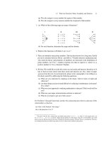
2. Troy is interested in skunks and has purchased a bevy of them to study. He plans to keep
the skunks in a rectangular skunk corral, as shown below. He will have a divider across
the width in order to separate the males and females. He has 510 meters of fencing to
make his corral.
(a) Let x = the width of the corral and y = the length of the corral. Use the fact that
Troy has only 510 meters of fencing to express y in terms of x.
(b) Express A, the total area enclosed for the skunks, as a function of x.
(c) Find the dimensions of the corral that maximize the total area inside the corral.
divider
x
y
3. The height of a ball (in feet) t seconds after it is thrown is given by
h(t) =−16t
2
+ 32t + 48 =−16(t + 1)(t − 3).
(a) Graph h(t) for the values of t for which it makes sense. Below it graph v(t).Be
sure that v(t) looks like the derivative of h(t).
(b) From what height was the ball thrown?

(c) What was the ball’s initial velocity? Was it thrown up or down? How can you tell?
(d) Was the ball’s height increasing or decreasing at time t = 2?
(e) At what time did the ball reach its maximum height? How high was it then? What
was its velocity at that time?
(f) How long was the ball in the air?
(g) What is the ball’s acceleration? Does this make physical sense?
242 CHAPTER 6 The Quadratics: A Profile of a Prominent Family of Functions
4. We know that Revenue = (price) · (quantity). Suppose a certain company has a mo-
nopoly on a good. If the company wants to increase its revenue it can do so by raising
its prices up to a certain point. However, at some point the price becomes so high that
there are not enough buyers and the revenue actually goes down. Therefore, if a mo-
nopolist is attempting to maximize revenue, the monopolist must look at the demand
curve. Suppose the demand curve for widgets is given by
p = 1000 − 4q,
where p is measured in dollars and q in hundreds of items.
(a) Express revenue as a function of price and determine the price that maximizes the
monopolist’s revenue.
(b) What price(s) gives half of the maximum revenue?
5. Suppose that q, the quantity of gas (in gallons) demanded for heating purposes, is given
by q = mp + b, where m and b are constants (m negative and b positive) and p is the
price of gas per gallon. The gas company is interested in its revenue function.
(a) Explain why m is negative.
(b) Express revenue as a function of price. (Note that m and b are constants, so if you
express revenue in terms of m, b, and p, you have expressed revenue as a function
of price.)
(c) Graph your revenue function, labeling all intercepts.
(d) From your graph, determine the price that maximizes revenue. (Your answer will
be in terms of m and b.)
(e) Find R


and graph it.
6. A catering company is making elegant fruit tarts for a huge college graduation cele-
bration. The caterer insists on high quality and will not accept shoddy-looking tarts.
When there are 7 pastry chefs in the kitchen they can each turn out an average of 44 tarts
per hour. The pastry kitchen is not very large; let us suppose that for each additional
pastry chef put to the fruit-tart task the average number of tarts per chef decreases by
4 tarts per hour. (Assume that reducing the number of chefs will increase the average
production by 4 tarts per hour, until the number of chefs has decreased to 3. At that
point reducing the number of chefs no longer increases the productivity of each chef.)
(a) How many chefs will yield the optimum hourly fruit-tart production?
(b) What is the maximal hourly fruit-tart production?
(c) How many chefs are in the kitchen if the fruit-tart production is 320 tarts per hour?
7. The function R(p) = 35p(75 − p) gives revenue as a function of price, p, where the
price is given in dollars.
(a) Find the price at which the revenue is maximum.
(b) What is the maximum price?
8. David and Ben are sitting in a tree house sorting through a basket of apples. They find
two that are rotten and decide to toss them into a garbage bin on the ground below.
The height of Ben’s apple t seconds after he throws it is given by
B(t) =−16t
2
+ 4t + 10,
6.4 The Free Fall of an Apple: A Quadratic Model 243
and the height of David’s apple t seconds after he throws it is given by
D(t) =−16t
2
− 2t + 10.
(a) From what height are the apples thrown?
(b) What is the maximum height of Ben’s apple? Explain your answer.
(c) What is the maximum height of David’s apple?

(d) Does Ben toss the apple up or throw it down? Does David toss the apple up or
throw it down? Explain your reasoning.
(e) How many seconds after he throws it does Ben’s apple hit the ground?
9. Amelia is a production potter. If she prices her bowls at x dollars per bowl, then she
can sell 120 − 5x bowls every week.
(a) For each dollar she increases her price how many fewer bowls does she sell?
(b) Express her weekly revenue as a function of the price she charges per bowl.
(c) Assuming that she can produce bowls more rapidly than people buy them, how
much should she charge per bowl in order to maximize her weekly revenue?
(d) What is her maximum weekly revenue from bowls?

7
CHAPTER
The Theoretical Backbone:
Limits and Continuity
7.1 INVESTIGATING LIMITS—METHODS OF INQUIRY
AND A DEFINITION
The idea of taking a limit is at the heart of calculus. The limiting process allows us to move
from calculating average rates of change to determining an instantaneous rate of change; in
other words, it allows us to determine the slope of a tangent line. We will need it to tackle
another fundamental problem in calculus, calculating the area under a curve. We’ve also
seen that the language of limits is useful as a descriptive tool.
Roots of the limiting processes can be found in the work of the ancient Greek mathe-
maticians. Archimedes essentially used a limiting process in studying the area of a circle,
calling his technique involving successive approximations “the method of exhaustion.” The
limiting process was instrumental in the work of Isaac Newton and Gottfried Leibniz as
they developed calculus and can also be found in work of their predecessors. It is inter-
esting that these early practitioners of calculus in the late 1600s achieved many useful and
valid results without carefully defining the notion of a limit. Not until substantially later
were mathematicians able to put the work of their predecessors on solid ground with a rig-

orous definition of a limit. While we will not work much with the rigorous definition, we
will use this chapter to put the notion of limit on more solid ground.
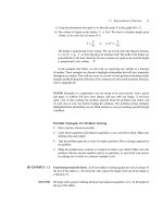
The challenge of computing instantaneous velocity from a displacement function,
s(t), led us to limits. To find the instantaneous velocity at, say, t = 3, we took successive
approximations using average velocity over the interval [3, 3 + h].
245
246 CHAPTER 7 The Theoretical Backbone: Limits and Continuity
(3, s(3))
(3 + h, s(3 + h))
∆t
∆ displacement
∆ time
∆s
s′(3) ≈
s(3 + h) – s(3)
h
s′(3) ≈
Figure 7.1
If h = 0 this expression is undefined; we have
0
0
. But the closer h is to zero the better the
approximation becomes. We are interested in what happens to
s(3+h)−s(3)
h
as h approaches
zero but is not equal to zero. This problem motivates our definition of limit.
What Do We Mean by the Word “Limit”?
Below we give a short answer, which we will expand upon throughout the section.
lim

x→2
f(x)=5means f(x)stays arbitrarily close to 5 provided that x is sufficiently
close to 2, but not equal to 2.
It does not tell us that f(2)=5. It gives us no information about f(2);f(2)could be
5, or
√
3, or undefined.
However, we can guarantee that the difference between f(x)and 5 is smaller than any
positive number, no matter how miniscule, if x is close enough to 2 (but not equal to
2).
lim
x→∞
f(x)=6means that the values of f(x)stay arbitrarily close to 6 provided x
is large enough.
lim
x→2
f(x)=∞means that f(x)increases without bound as x approaches 2.
We’ll clarify the meaning of “arbitrarily close to” through the next two examples.
◆
EXAMPLE 7.1 Argue convincingly that if g(x) =
1
x
, then lim
x→∞
g(x) =0.
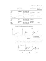
SOLUTION It “appears,” from the graph of g(x) =
1
x
(see Figure 7.2), that lim
x→∞

1
x
= 0; numerical
evidence suggests this hypothesis as well.
g
g(x) =
x
x
1
g(x) =
x
x
1
10
100
1000
10000
10
5
10
6
.1
.01
.001
.0001
10
–5
10
–6
Figure 7.2

7.1 Investigating Limits—Methods of Inquiry and a Definition 247
But appearances alone can be deceiving. For instance, suppose we graph h(x) =
1
x
+ 10
−15
.
Adding 10
−15
to g(x) shifts the graph of g(x) vertically up by 10
−15
. But 10
−15
is such a
miniscule number that it is difficult to distinguish between h and g graphically (particularly
using a graphing calculator). Yet if lim
x→∞
1
x
= 0 then lim
x→∞
(
1
x
+ 10
−15
) ought to be
10
−15
. So although the graph in Figure 7.2 is very useful, it isn’t convincing evidence that

lim
x→∞
1
x
= 0.
The table of values suggests a way of nailing things down. Since
1
x
is positive and
decreasing, we see that
g(x) is within 10
−5
of zero provided x>10
5
,
g(x) is within 10
−6
of zero provided x>10
6
,
g(x) is within 10
−100
of zero provided x>10
100
.
Even this last statement is not enough to show that lim
x→∞
g(x) = 0. We must show that
g(x) will be arbitrarily close to zero for all x large enough. This means someone can issue
a challenge with any miniscule little number. Let  (read: epsilon) be any small positive

number;  can be excruciatingly small. We must show that for x large enough, g(x) is
within  of 0.
g(x) =
1
x
is within  of zero provided x>
1

.
We’re done.
◆
In our next example we’ll look at lim
x→∞

1
2

x
.
Before launching in, first we note that we define

1
2

n
for n a positive integer as
1
2
multiplied by itself n times:
1

2
·
1
2
·
1
2

1
2

 
n times
.
Using the rules of exponent algebra, which can be reviewed in either the Algebra Appendix
or Chapter 9 for any rational exponent x, we can define

1
2

x
for x any rational number.
For now we’ll deal with irrational exponents simply by approximating the irrational number
by a sequence of rational ones. Suppose x is irrational, r and s are rational, and r<x<s.
Then

1
2

r

<

1
2

x
<

1
2

s
.Wedefine b
x
so as to make the graph of b
x
continuous. A more
satisfactory definition can be given after taking up logarithmic functions.
◆
EXAMPLE 7.2 Argue convincingly that lim
x→∞

1
2

x
= 0.
SOLUTION Let’s begin by trying to get a feel for what happens to
1
2

x
as x increases without bound.
Consider the graph of f(x)=

1
2

x
=
1
2
x
on the following page.
248 CHAPTER 7 The Theoretical Backbone: Limits and Continuity
f
x
1
Figure 7.3
A second way of getting a feel for the limit is to look numerically at the outputs of
f(x)=
1
2
x
as x gets increasingly large.
x f (x) =
1
2
x
= (0.5)
x

(approximate values)
20 9.5 × 10
−7
= 0.00000095
50 8.8 × 10
−16
= 0.00000000000000088
100 7.8 × 10
−31
200 6.2 × 10
−61
300 4.9 × 10
−91
It “appears” that lim
x→∞
1
2
x
= 0. This is looking quite convincing; 4.9 × 10
−91
is quite
close to zero. But consider the following. When asked to compute 0.5
328
, a TI-81 calculator
gives approximately 1.8 × 10
−99
. But when asked for 0.5
329
, it gives the answer as 0. In
fact, according to this calculator, for x>329,

1
2
x
= 0. We know this is false; a fraction can
be equal to zero only if its numerator is zero, and here the numerator is 1. It appears that
the calculator rounds 10
−100
off to zero. How can we be sure that lim
x→∞
1
2
x
= 0, and not
10
−120
for instance? It is not quite good enough to simply say 0 <f(x)<10
−99
provided
x>330.
1
As in Example 7.1, we must show that f(x)will be arbitrarily close to zero provided
that x is large enough. Again, a challenge is issued with any excruciatingly small number
; we must show that f(x)is within  of 0 for x big enough. To figure out how big is “big
enough,” let’s compare f(x)=
1
2
x
with g(x) =
1
x

.
1
This statement is true because as x increases f(x)decreases.
7.1 Investigating Limits—Methods of Inquiry and a Definition 249
y
g(x) =
x
x
1
f(x) =
f(x) =
x
(approximated)
1
2
x
1
2
g(x) =
x
x
1
20
50
100
200
.05
.02
.01
.005

9.5 × 10
–7
8.8 × 10
–16
7.8 × 10
–31
6.2 × 10
–61
Figure 7.4
Notice that
1
2
x
<
1
x
for all x>0.(This is equivalent to the statement that if x>0,then
2
x
>x.)
So for x>0, if
1
x
is within  of zero, then
1
2
x
is certainly within  of zero.
And
1

2
x
is within  of zero provided x>
1

. (Notice by looking at the table of values that
for large x,
1
2
x
is much, much smaller than
1
x
, so requiring that x>
1

is overkill—but
that’s all right.)
◆
The last two examples highlight a couple of important ideas about limits in general and
lim
x→∞
f(x)=Lin particular:
1. Graphical and numerical investigations are both useful methods of inquiry that can
provide compelling data from which to arrive at a conjecture about a limit. They cannot,
however, be conclusive on their own.
2. When we say “f(x)is arbitrarily close to L” we mean that the distance between f(x)
and L can be made arbitrarily small. To be arbitrarily small means that we can answer
a challenge set out by any miniscule positive number , no matter how excruciatingly
small  may be, that the distance between f(x)and L can be made less than  given

certain conditions on x.
◆
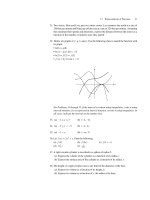
EXAMPLE 7.3 Find lim
x→3
x
2
.
SOLUTION Very loosely speaking, this problem asks “what does f(x)=
x
2
approach as x gets closer
and closer to 3 but is not equal to 3?” Intuitively, it should make sense that lim
x→3
x
2
= 1.5.
There is nothing particularly special happening to
x
2
around x = 3.
f
f(x) =
x
x
2
2
3
x
x
2

2.9
2.99
2.999
2.99999
3.00001
3.001
3.01
3.1
1.45
1.495
1.4995
1.499995
1.500005
1.5005
1.505
1.55
3
Figure 7.5
250 CHAPTER 7 The Theoretical Backbone: Limits and Continuity
More rigorously, we can show that if x is close enough to 3 (but not equal to 3), then
x
2
can
be made to stay arbitrarily close to 1.5 as follows.
Look at Figure 7.6(a). We can see that if x is within 1 unit of 3, then f(x) is within
0.5 units of 1.5. Similarly, we see in Figure 7.6(b) that if x is within 0.1 of 3, then f(x)is
within 0.05 =
0.1
2
of 1.5.

f
f(x) =
x
x
2
342
1
1
2
1
f
f(x) =
x
x
2
1.55
1.5
1.45
.1
2
= .05
.05
2.9 3 3.1
(a) (b)
Figure 7.6
Because f(x)is a straight line with slope 1/2, we can see that the ratio
f
x
is always
0.5. We use this to ensure that the distance between f(x) and 1.5 can be made arbitrarily

small for x close enough to 3 but x = 3.
For  any positive number, no matter how excruciatingly small, if x is within 2 of 3
(x = 3), then f(x)will be within  of 1.5. Therefore lim
x→3
x
2
= 1.5.
◆
This last example illustrates what we mean by lim
x→3
f(x)=L.Showing that f(x)
stays arbitrarily close to L for x close enough to 3 (but not equal to 3) is equivalent to the
following: Given the challenge of any excruciatingly small positive , we can guarantee
that f(x) will be within  of L provided x is close enough to 3. We can write this more
compactly: If f(x)is within  of L, then the distance between f(x)and L is less than .
Let’s use absolute values to express this distance.
The distance between f(x)and L is |f(x)−L|.
Similarly, the distance between x and3is|x−3|.
Toshow that x is within some distance δ (delta for distance) of 3 but not equal to 3, we
write 0 < |x − 3| <δ.
Wearrive at the following definition, which we use in the examples which follow.
Definition
lim
x→3
f(x)=Lif, for every excruciatingly small positive number , we can come
up with a distance δ so that
|f(x)−L|<provided 0 < |x − 3| <δ.
This is the formal definition of a limit
2
(where we can substitute “a” for 3 to get

lim
x→a
f(x)=L). We applied this definition in the last example. As promised at the
2
f must be defined on an open interval around 3, although not necessarily at x = 3.