Calculus: An Integrated Approach to Functions and their Rates of Change, Preliminary Edition Part 38 docx

10.1 Analysis of Extrema 351
f
x
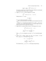
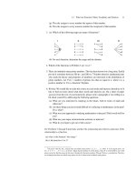
(i) f(x) = |x| on (–∞, ∞)
f
x
(ii) f(x) = x on [–1, 2]
–1 2
Figure 10.12
Local Extrema
Suppose x = c is an interior critical point of a continuous function f . How can we tell if,
at x = c, f has a local maximum, local minimum, or neither?
One approach is to look at the sign of f

to determine whether f changes from
increasing to decreasing across x = c. This type of analysis is referred to as the first
derivative test. If f is continuous, x = c is an interior critical point of f , and f is
differentiable on an open interval around c (even if f is not differentiable specifically at
c), then:
if f

changes sign from negative to positive at x = c, then f has a local minimum at c;
if f

changes sign from positive to negative at x = c, then f has a local maximum at c;
if f

does not change sign across x = c, then f does not have a local extremum at c.
graph of f
sign of f′
local min at c local max at c

graph of f
sign of f′
c– +
c –+
Figure 10.13
Suppose x = c is an interior critical point of f but f is not continuous. You might wonder
if there is a first derivative test we can apply. The answer is no. Look carefully at the graphs
presented in Figure 10.14.
k
x
1
–1
f
x
Figure 10.14
Global Extrema
Suppose we’ve rounded up theusual suspects for extrema; we’ve identified the critical points
of f . Is there an easy way to identify the global maximum and minimum values? First we
have to figure out whether or not the function has a global maximum. If we know it does,
352 CHAPTER 10 Optimization
we can calculate the value of the function at each of the critical points. The largest value is
the global maximum value. (The corresponding x gives you the absolute maximum point.)
Sometimes you can exclude a few candidates. For instance, a local minimum will never be
a global maximum.
Critical point xf(x)
Compare the
values of f
at its critical
points.
List all critical

points of f.
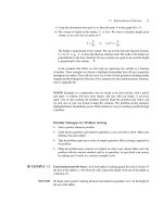
Some functions don’t have absolute maximum and minimum values. Think about the
functions f(x)=1/x and h(x) = x
2
, each on its natural domain. The former has neither
a maximum nor a minimum and the latter has only a minimum. Or consider g(x) = x and
h(x) = x
2
on the interval (0, 1). On this open interval neither of these functions has a global
maximum or a global minimum.
g
x
(b) g(x) = x on (0, 1)
f
x
(a) f(x) = 1/x (c) h(x) = x
2
on (0, 1)
h
x
1
Figure 10.15
Think about what went wrong in the cases above and see what criteria might guarantee
a global extrema. To begin with, let’s look at a function whose domain is a closed inter-
val, [a, b]. This will fix the problems encountered in the case of functions f , g, and h
above.
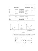
Now consider the functions j(x)=
1
x
for x = 0 and 0 for x = 0ork(x ) = (x

2
) for x = 0
and 1 for x = 0, both restricted to the closed interval [−1, 1]. (See Figure 10.16.) To rule
out these cases, we insist that the function be continuous. A continuous function on a closed
interval is guaranteed to attain an absolute maximum value and an absolute minimum value.
This is the Extreme Value Theorem discussed in Chapter 7. (It should seem reasonable, but
its proof is difficult and beyond the scope of this text.)
10.1 Analysis of Extrema 353
k
x
1
–1
Figure 10.16
Summary
If f has any local or global extrema, these will occur at critical points of f . x
0
is a
critical point of f if x
0
is in the domain of f , and:
f

(x
0
) = 0, or
f

(x
0
) is undefined, or

x
0
is an endpoint of the domain of f .
Absolute extrema: If f is continuous on a closed interval [a, b], then f attains an
absolute maximum and absolute minimum on [a, b] (Extreme Value Theorem). These
can be found by evaluating f at each of its critical points. Where the value of f is
greatest, f has an absolute maximum; where the value of f is least, f has an absolute
minimum. When looking for absolute extrema in general, you must treat the situations
on a case-by-case basis. Stand back and take a bird’s-eye view of the function to see if
you expect global extrema. If f has any absolute maximum or minimum values, they
will occur at the critical points.
Local extrema: Suppose x
0
is a critical point of f .Iff is continuous at x
0
and f

exists
in an open interval around x
0
, although not necessarily at x
0
itself, then we can apply the
first derivative test. If the sign of f

changes at x
0
, then f has a local extremum at x
0
.

Plot sign information on a number line to distinguish between maxima and minima. If
the sign of f

does not change on either side of x
0
, then f has neither a local maximum
nor a local minimum at x
0
.
◆
EXAMPLE 10.4 Let f(x)=x
3
−12x + 3. Find all local extrema of f .
SOLUTION Look for critical points.
f

(x) = 3x
2
− 12
f

is defined everywhere, and the function is defined for all real numbers, therefore the only
critical points are the zeros of f

.
f

(x) = 3x
2
− 12 = 0

3(x
2
− 4) = 0
x =±2.
To determine whether these points are extrema, we set up a number line and determine
the sign of f

in each of the three intervals into which the critical points partition the line.
354 CHAPTER 10 Optimization
–2
(+) (+)(–)
graph of f
sign of f ′
2
So f has a local minimum at x = 2 and a local maximum at x =−2. ◆
◆
EXAMPLE 10.5 Suppose f is continuous on (−∞, ∞). f

= 0atx=−1and at x = 2. f

does not exist at
x =−3and at x = 0. Classify the critical points of f as best you can given the information
below regarding the sign of f

.
–3
–1 20
00
(+) (+) (–)(–)(–)
sign of f′

f ′ undef. f ′ undef.
SOLUTION Correlating the sign of the derivative with information about the slope of the function gives
us the following number line.
–3
–1 20
(+) (+) (–)(–)(–)
graph of f
sign of f ′
This gives us the following information about the extrema of f :
at x =−3, f has a local maximum;
at x =−1, f has a local minimum;
at x = 0, f has a local maximum;
at x = 2, f has neither a local maximum nor minimum.
There is not enough information to determine whether or not f has an absolute minimum
value. It has an absolute maximum at either x =−3orx=0,or at both. There is not enough
information to make a stronger statement.
◆
PROBLEMS FOR SECTION 10.1
In Problems 1 through 16, for each function:
(a) Find all critical points on the specified interval.
(b) Classify each critical point: Is it a local maximum, a local minimum, an absolute
maximum, or an absolute minimum?
(c) If the function attains an absolute maximum and/or minimum on the specified
interval, what is the maximum and/or minimum value?
1. f(x)=x
3
−3x+2on(−∞, ∞)
2. f(x)=x
3
−3x+2on[−5, 5]

3. f(x)=x
3
−3x+2on[0, 3]
10.1 Analysis of Extrema 355
4. f(x)=x
3
−3x+2on(0, 3)
5. f(x)=−2x
3
+3x
2
+12x + 5on(−∞, ∞)
6. f(x)=−2x
3
+3x
2
+12x + 5on[−3, 4]
7. f(x)=x
5
−20x + 5on(−∞, ∞)
8. f(x)=x
5
−20x + 5on[−2, 0]
9. f(x)=x
5
−20x + 5 on [0, 2]
10. f(x)=3x
4
−8x
3

+3on(−∞, ∞)
11. f(x)=3x
4
−8x
3
+3on[−1, 1]
12. f(x)=3x
4
−8x
3
+3on(0, 3)
13. f(x)=
x
3
3
+ 2x +
3
x
on its natural domain. Why is x = 0 not a critical point?
14. f(x)=
x
3
3
+ 2x +
3
x
on [−3, 0)
15. f(x)=
x
3

3
+ 2x +
3
x
on (0, 3]
16. f(x)=
1
x
2
+4
on (−∞, ∞)
17. Let f(x)=
e
x
x
.
(a) Find all critical points of f .
(b) Identify all local extrema.
(c) Does f have an absolute maximum value? If so, where is it attained? What is its
value?
(d) Does f have an absolute minimum value? If so, where is it attained? What is its
value?
(e) Answer parts (c) and (d) if x is restricted to (0, ∞).
18. Let f(x)=x
2
e
−x
.
(a) Find all critical points of f .
(b) Classify the critical points.

(c) Does f take on an absolute maximum value? If so, where? What is it?
(d) Does f take on an absolute minimum value? If so, where? What is it?
In Problems 19 through 26, find and classify all critical points. Determine whether or
not f attains an absolute maximum and absolute minimum value. If it does, determine
the absolute maximum and/or minimum value.
19. f(x)=(x
2
− 4)e
x
356 CHAPTER 10 Optimization
20. f(x)=
10x
x
2
+1
21. f(x)=
10x
2
x
2
+1
22. f(x)=
x
e
x
23. f(x)=
x−1
x
2
+3

24. f(x)=
4−x
x
2
+9
25. f(x)=
x
3
x
2
+1
26. f(x)=
e
x
2x
10.2 CONCAVITY AND THE SECOND DERIVATIVE
In this section we will take another look at concavity to see what it can tell us when we are
analyzing critical points. Recall that where f

is increasing the graph of f is concave up,
and where f

is decreasing the graph of f is concave down. Let’s see what bearing this has
on optimization.
Suppose x
0
is a stationary point: f

(x
0

) = 0. Then f has a horizontal tangent line at
x = x
0
.
If f

is increasing at x
0
, then locally the graph must look like Figure 10.17(a);
f has a local minimum at x
0
.
If f

is decreasing at x
0
, then locally the graph must look like Figure 10.17(b);
f has a local maximum at x
0
.
(x
0
, f(x
0
))
(x
0
, f(x
0
))

(a) (b)
Figure 10.17
We know that
f

> 0 ⇒ f

is increasing ⇒ f is concave up;
f

< 0 ⇒ f

is decreasing ⇒ f is concave down.
or
or
or
or
Therefore, if f

(x
0
) = 0 and f

(x
0
) exists, we can look at the sign of f

(x
0
) and draw the

following conclusions:
10.2 Concavity and the Second Derivative 357















If f

(x
0
)>0, then f is concave up around x
0
and therefore has a local minimum
at x
0
.
If f

(x

0
)<0, then f is concave down around x
0
and therefore has a local maximum
at x
0
.
If f

(x
0
) = 0, we cannot draw any conclusions. The function could have a maximum
at x
0
, a minimum at x
0
, or neither.
This set of criteria is referred to as the second derivative test.
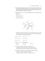
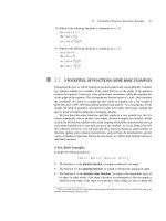
EXERCISE 10.1 Look at the case where f

(x
0
) = 0 and f

(x
0
) = 0. In the three examples below, determine
whether the function has a maximum at x
0
= 0, a minimum at x

0
= 0, or neither a maximum
nor a minimum at x
0
= 0. Sketch the graphs of these functions on the set of axes provided
below as an illustration of why f

(x
0
) = 0 and f

(x
0
) = 0 does not allow us to classify x
0
.
f
x
(ii) f(x) = x
4
f
x
(iii) f(x) = –x
4
f
x
(i) f(x) = x
3
Figure 10.18
Definition

A point of inflection is a point in the domain of f at which f changes concavity,
i.e., a point at which f

changes sign.
CAUTION The fact that f

(x
0
) = 0 does not necessarily mean that x = x
0
is an inflection
point. Look back at the graphs you’ve drawn in Exercise 10.1. x = 0 is a point of inflection
for f(x)=x
3
butnot for f(x)= x
4
.
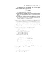
f
x
1
2 3 4–1–2–3
x = –2, x = –1, x = 1 and
x = 3.5 are all points
of inflection.
Figure 10.19
Putting It All Together
Suppose x = 3 is an interior critical point of a continuous function f and we are interested
in classifying this critical point, that is, in determining whether x = 3 is a local maximum,
a local minimum, or neither. What can we do?
358 CHAPTER 10 Optimization

Method (i) First Derivative Test.
We can look at the sign of f

, the first derivative, on either side of 3. If f

changes sign
around 3, then 3 is a local maximum or local minimum point.
Method (ii) Second Derivative Test.
If f

(3) = 0, then we can look at the sign of f

(3).
If f

(3)>0,then f has a local minimum at x = 3.
If f

(3)<0,then f has a local maximum at x = 3.
If f

(3) = 0, we have insufficient information to draw a conclusion. In this case, turn
to method (i).
3
3
If x
0
is an endpoint, then the only label it can get is absolute maximum or absolute
minimum; otherwise it remains without a label. By looking at the sign of f


in the vicinity
of x
0
we can determine whether it is a potential absolute maximum or potential absolute
minimum. We need a bird’s-eye view to determine whether there is an absolute extremum.
If we expect one, we must compare the value of f at x
0
with its value at other candidates.
The first derivative test is widely applicable. It requires determining the sign of f

on intervals. Because the second derivative test only requires evaluating f

at a point, it
is simple to apply if f

is easy to calculate. For instance, consider Example 10.3 where
V(x)=4x
3
−48x
2
+ 144x, V

(x) = 12x
2
− 96x + 144 and V

(x) = 24x − 96. The only
interior critical point of V on [0, 6] is x = 2, and V

(2) = 24 × 2 − 96 < 0. We conclude

that V has a local max at x = 2. The second derivative test, however, can only be applied at
a point at which the first derivative is zero, i.e., at a stationary point. The graphs in Figure
10.20 illustrate why this is the case.
x
0
x
0
x
0
f " > 0 except at
the critical point
f " < 0 except at
the critical point
f " changes sign
at the critical point
concavity gives us no
useful information on
classifying endpoints
Figure 10.20 The second derivative test can’t be applied unless f

= 0 at the critical point.
f positive / negative increasing /decreasing concave up / concave down
f

positive / negative increasing /decreasing
f

positive / negative
PROBLEMS FOR SECTION 10.2
In Problems 1 through 12:

(a) Find all critical points.
10.2 Concavity and the Second Derivative 359
(b) Find f

. Use the second derivative, wherever possible, to determine which critical
points are local maxima and which are local minima. If the second derivative test
fails or is inapplicable, explain why and use an alternative method for classifying
the critical point.
1. f(x)=x
3
−6x+1
2. f(x)=−x
3
+3π
2
x
3. f(x)=x
3
+
9
2
x
2
− 12x +
3
2
4. f(x)=x
5
−5x
5. f(x)=2x

4
+64x
6. f(x)=x
6
+x
4
7. f(x)=x
4
+4x
3
+2
8. f(x)=4x
−1
+2x
2
9. f(x)=e
x
−x
10. f(x)=xe
x
−e
x
11. f(x)=
x
5
5
− x
4
+
4

3
x
3
+ 2
12. f(x)=3x
4
−8x
3
+6x+1
13. Suppose that f is a continuous function and that f(3)=2, f

(3) = 0, and f

(3) = 3.
At x = 3, does f have a local maximum, a local minimum, neither a local maximum
nor a local minimum, or is it impossible to determine? Explain your answer.
14. Suppose that f is a continuous function and that f(4)=1, f

(4) = 0, and f

(4) = 0.
At x = 4, f could have a local maximum, a local minimum, or neither. Sketch three
graphs, all satisfying the conditions given, one in which f has a local minimum at
x = 4, one in which f has a local maximum at x = 4, and one in which f has neither
a local maximum nor a local minimum at x = 4.
15. Without using the graphing capabilities of your graphing calculator, sketch the follow-
ing graphs. Label the x-coordinates of all peaks and valleys. Label exactly, not using
a numerical approximation. (If the x-coordinate is
√
2, it should be labeled

√
2, not
1.41421.)
Below the sketch of f , sketch f

(x), labeling the x-intercepts of the graph of f

.
(You can use your graphing calculator to check your answers.)
(a) f(x)=x(x −9)(x − 3) (Start by looking at the x-intercepts. Then look at the sign
of f

(x) in order to determine where the graph of f is increasing and where it is
decreasing.)
360 CHAPTER 10 Optimization
(b) f(x)=−2x(x −9)(x − 3) (Conserve your energy! Think!)
(c) f(x)=−2x(x −9)(x − 3) + 18 (Conserve your energy! Think!)
16. (a) The function g with domain (−∞, ∞) is continuous everywhere. We are told that
g

(
√
5) = 0. Some of the scenarios below would allow us to conclude that g has a
local minimum at x =
√
5. Identify all such scenarios.
i. g(
√
5) = 0, g(2) = 1, g(3) = 1
ii. g(

√
5)<0and g

(x) > 0 for x>
√
5.
iii. g

(
√
5)>0
iv. g

(
√
5)<0
v. g

(x) > 0 for x<
√
5 and g

(x) < 0 for x>
√
5
vi. g

(x) < 0 for x<
√
5 and g


(x) > 0 for x>
√
5
vii. g

(
√
5)>0and g

(
√
5) = 0
(b) The function h with domain [−8, −3] has the following characteristics.
h is continuous at every point in its domain.
h

(x) < 0 for −8 <x<−4and h

(x) > 0 for (−4, −3).
h

(−4) is undefined.
What can you conclude about the local and absolute extrema of h? Please say as
much as you can given the information above.
17. The graph of f

(not f ,butf

)isaparabola with x-intercepts of −π and 2π and a

y-intercept of −2.
(a) Draw a graph of f

.
(b) Write an equation for f

. This equation should have no unknown constants.
(c) On the graph you drew in part (a), go back and label the x- and y-coordinates of
the vertex.
(d) Find f

(x).
(e) This part of the question asks about f , not f

.
i. Where does f have a local maximum? Explain your reasoning clearly and
briefly.
ii. Where does f have a local minimum? Explain your reasoning clearly and
briefly.
iii. Does f have an absolute maximum or minimum value? Explain.
iv. The function f has a single point of inflection. What is the x-coordinate of
this point of inflection? Suppose you are told that the y-coordinate of the point
of inflection is −1. Find the equation of the tangent line to the graph of f at
its point of inflection.
18. Consider the function f(x)=x
5
−2x
4
−7 restricted to the domain [−1, 1]. Your
reasoning for the questions below must be fully explained and be independent of a

graphing calculator.
(a) Find the absolute maximum value of f(x)on the interval [−1, 1] or explain why
this is not possible.
(b) Find the absolute minimum value of f(x)on the interval [−1, 1] or explain why
this is not possible.
(c) Find the absolute minimum value of f(x)on the open interval (−1, 1) or explain
why this is not possible.