Calculus: An Integrated Approach to Functions and their Rates of Change, Preliminary Edition Part 42 pps

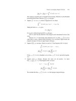
11.3 Polynomial Functions and Their Graphs 391
11.3 POLYNOMIAL FUNCTIONS AND THEIR GRAPHS
Graphing Polynomials
We’ll begin with a couple of examples and then arrive at a general strategy for understanding
the graphs of polynomials.
◆
EXAMPLE 11.6 Graph f(x)=x
3
−2x
2
−8x,identifying the x-coordinates, all zeros, local extrema, and
inflection points.
SOLUTION Zeros. This is the function from Example 11.2. In factored form f(x)=x(x −4)(x +2);
it has zeros at x =−2, x = 0, and x = 4. The graph of f(x) does not cross the x-axis
anywhere between these zeros. f is continuous, so its sign can’t change between the zeros.
Therefore, between x =−2and x = 0, for example, f(x)must be always positive or always
negative. By determining the sign of f(x)for just one test value of x on the interval (−2, 0),
we can determine the sign of f(x) on the entire interval (−2, 0). We draw a number line
showing the zeros of f(x)and the sign of f(x)between those zeros.
Sign Computations—suggested method: Work with f in factored form:
f(x)=x(x −4)(x + 2).We’ll start with x very large and then look at the effect on the sign
of the factors as x decreases and passes by each zero.
00 0
(–) (+) (+)(–)
–240
Sign of f
For x very large, all factors are positive: (+)(+)(+) ⇒ (+)
As x drops below 4, the factor (x − 4) changes sign: (+)(−)(+) ⇒ (−)
As x drops below 0, the factor x changes sign: (−)(−)(+) ⇒ (+)
As x drops below −2, the factor (x + 2) changes sign: (−)(−)(−) ⇒ (−)
A spot-check can be used to confirm this.

4–2
y
x
Figure 11.10
Local Extrema. We need to look at the first derivative to determine critical points: f

(x) =
3x
2
− 4x − 8. We use the quadratic formula to determine where f

(x) = 0 and obtain
x =
2+2
√
7
3
≈2.43, and x =
2−2
√
7
3
≈−1.10. By drawing a number line showing these points
where f

(x) = 0 and indicating the sign of f

(x) between them, we can determine whether
these stationary points are local minima, local maxima, or neither.
392 CHAPTER 11 A Portrait of Polynomials and Rational Functions

graph of f(x)
sign of f ′(x)
2 – 2√7
3
2 + 2√7
3
(+) (+)(–)
Computations:
If x is large enough in magnitude, x
2
dominates and f

is positive.
For x = 2/3 (between the zeros) f

is negative.
So, f(x)has a local maximum at x =
2−2
√
7
3
and a local minimum at x =
2+2
√
7
3
.
We know that a cubic on a nonrestricted domain will have neither a global maximum
value nor a global minimum value; when the domain of a cubic is (−∞, ∞), the range is
also (−∞, ∞).

Inflection Points. Take the second derivative: f

(x) = 6x − 4. f

(x) = 0 when x = 2/3.
We draw another number line to show the sign of f

(x) and the corresponding concavity
of f(x).
concave down concave up
(–) (+)
2
3
concavity of f(x)
sign of f ″(x)
All this information taken together enables us to draw an accurate graph of f(x).
y
x
5
3
4–2
2–2√7
3
2+2√7
3
2
f(x)
Figure 11.11
◆
◆

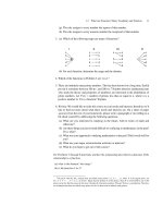
EXAMPLE 11.7 Sketch a rough graph of f(x)=−(x + 3)(x − 2)
2
, labeling all zeros and showing where
f(x) is positive and where f(x) is negative. See how much information can be gotten
without using derivatives.
SOLUTION The cubic f(x) has only two zeros: a zero at x =−3and a double zero at x = 2. As in
Example 11.6, let’s draw a number line showing the zeros of f(x)and the sign of f(x)in
between these zeros.
2–3
y
x
Figure 11.12
11.3 Polynomial Functions and Their Graphs 393
Notice that here f(x)does not change sign when it passes through the zero at x = 2; it is
negative on both sides of this zero. This is because the (x − 2)
2
term in f(x)doesn’t change
sign when x passes through x = 2.
y
x
2–3
f(x)
Figure 11.13
f has a local maximum at x = 2. To find the local minimum, we would need to calculate
f

. Do this as an exercise.
◆
Can you figure out in general what effect multiple (double, triple, or higher) roots have
on the graph of f(x)?(Hint: Consider separately the cases where the factor (x − a) is raised

to even and odd powers and analyze the sign.)
Strategy for Graphing a Polynomial Function f
1. Bird’s-eye view
Look at the degree of the polynomial and the sign of the leading coefficient to anticipate
what is ahead. From this information, determine whether the polynomial will have a
global maximum or a global minimum or neither.
2. Positive/negative
x-intercepts are simple to find if we can factor the polynomial into linear and quadratic
factors. In theory this is always possible, but in practice it may be very difficult.
Polynomials are continuous functions, so if P(x) changes sign between x = a and
x = b there must be at least one x-intercept between x = a and x = b.Ifyoufind the
x-intercepts, plot them. If you are certain you’ve identified all the zeros of P(x), then
check the sign of P(x)in each interval.
5
Note: If the x-intercepts are symmetrically placed, check for even or odd symmetry.
If x is only raised to even powers, the graph will be symmetric about the y-axis. If x
is only raised to odd powers and there is no constant term, then the graph will be
symmetric about the origin.
y-intercept: P(0)
3. Increasing/decreasing
Look at the sign of P

(x). On a number line plot the points where P

(x) = 0 and then
check the sign in every interval.
P

> 0 ⇒ the graph of P is increasing
P


< 0 ⇒ the graph of P is decreasing
5
If the polynomial is in factored form, it’s easy to check the sign of the polynomial at, say, x = 3, by checking the sign of
each of the factors at x = 3 and then “multiplying the signs” together.
394 CHAPTER 11 A Portrait of Polynomials and Rational Functions
Since P

is continuous, P

= 0 at any turning point (local maximum or minimum) of
the graph.
Note: If P

(3) = 0 we cannot conclude that the graph must have a local maximum or
minimum at x = 3. We can only be sure that the graph has a horizontal tangent line at
x = 3. P will have a local extrema at x = 3 only if P

changes sign at x = 3.
4. Concavity—fine tuning Look at the sign of P

(x). On a number line plot the points
where P

(x) = 0 and check the sign in every interval.
P

> 0 ⇒ the graph of P is concave up
P


< 0 ⇒ the graph of P is concave down
Note: P will have a point of inflection at x = c only if P

changes sign at x = c.
5. Look back at what you’ve done. Consider the degree of the polynomial and make sure
that your graph makes sense.
A graphing calculator or computer can be useful for graphing polynomials. For in-
stance, if zeros are hard to find a machine is useful in approximating them. It is up to you,
however, to determine an appropriate viewing window.
◆
EXAMPLE 11.8 Graph
6
P(x)= 100x
4
− 900x
2
.
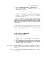
SOLUTION 1. P(x)is a fourth degree polynomial with a positive leading coefficient, so from a bird’s-
eye view the graph should look something like

At the extremities the graph reaches upward. The graph must have either one or three
turning points.
7
2. P(x)= 100x
4
− 900x
2
= 100x
2
(x

2
− 9) = 100x
2
(x + 3)(x − 3)
The x-intercepts are therefore at x = 0, x = 3, and x =−3. (Plot these zeros.)
The x-intercepts are symmetrically located, so we check for symmetry. All x’s are
raised to even powers, so P(−x) = P(x).This means the graph has even symmetry; it
is symmetric about the y-axis.
3. P(x)= 100(x
4
− 9x
2
),soP

(x) = 100(4x
3
− 18x) = 200x(2x
2
− 9).
6
Try to graph this on your graphing calculator. You’ll probably find that it takes you some time to find a suitable viewing
window.
7
This follows from the previous statement. The derivative of a fourth degree polynomial is a cubic, which can have one, two,
or three zeros, but the cubic will change sign either once, or three times.
Fourth degree polynomial Third degree polynomial
or
y
x
y

x
y
x
11.3 Polynomial Functions and Their Graphs 395
3–3
p
x
P

(x) = 0atx=0and where 2x
2
− 9 = 0, i.e., x
2
=
9
2
,orx=±
3
√
2
.
graph of P
sign of P′
(–) (+) (–) (+)
0
–3
√2
3
√2
There are local minimum points at x =

3
√
2
and at x =−
3
√
2
and a local maximum at
x = 0.
P(x)=100x
2
(x
2
− 9),so
P(0)=0
P

3
√
2

= 100

9
2

9
2
− 9


= 450

−
9
2

=−2025.
Likewise,
P

−
3
√
2

=−2025.
4. P

(x) = 100(12x
2
− 18) = 200(6x
2
− 9)
P

(x) = 0 provided that
6x
2
= 9
x

2
=
9
6
x
2
=
3
2
x =±

3
2
.
graph of P
sign of P″
(+) (–)
–
(+)
3
2
3
2
concave
up
concave
up
concave
down
√

√
First, using the information we have gathered, try to draw the graph yourself. Now use a
graphing calculator or computer to check your answer. Notice that you have to be careful
about your choice of range and domain, otherwise the machine will be of little help.
396 CHAPTER 11 A Portrait of Polynomials and Rational Functions
–3
√2
3
√2
–
3
2
√
3
2
√
P
x
x = x =
–33
Figure 11.14
◆
EXERCISE 11.8 Consider the polynomial f(x)=100x
4
− 900x
2
− 2.
(a) How many zeros does f(x)have? (Use the results of Example 11.8 to aid you.)
(b) Approximately where are the zeros? (Give your answers to within 0.01.)
(c) Show that 3 is not a zero of f(x).Isthe zero in the vicinity of 3 larger than 3 or smaller

than 3? Explain your reasoning.
Answer
There are two zeros near x =±3. In actuality, one is between 3.00031 and 3.00052, and
the other is between −3.00031 and −3.00052.
EXERCISE 11.9 Graph y = 100x
4
− 900x
2
+ 800. (Hint: Factor this first into two quadratics, then factor
the quadratics themselves.)
Finding a Polynomial Function to Fit a Polynomial Graph
◆
EXAMPLE 11.9 Find a function to fit the cubic function f(x)shown.
–2
1
(2, –5)
x
y
f(x)
Figure 11.15
SOLUTION We see that f(x)has zeros at x =−2, x = 0, and x = 1, so f(x)must have factors (x + 2),
x, and (x − 1). Since it is a cubic, we can write
f(x)=k(x + 2)(x)(x − 1).
11.3 Polynomial Functions and Their Graphs 397
Multiplying by the constant k does not change the location of any of the x-intercepts (since it
rescales vertically), but it does allow us to ensure that f(x)passes through the point (2, −5)
as it does in the graph. Knowing that x = 2, y =−5must satisfy the equation gives us
−5 = k(2 + 2)(2)(2 − 1)
−5 = 8k
k =−

5
8
.
The equation must be f(x)=−
5
8
(x + 2)(x)(x − 1). You can verify this on your graphing
calculator.
◆
◆
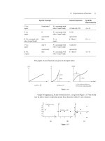
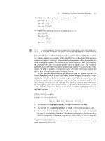
EXAMPLE 11.10 Find a possible equation for the polynomial function g(x ) shown.
–1
–1.5
–2
1 2 3
–10
g(x)
x
y
Figure 11.16
SOLUTION g(x ) has three zeros, at x =−1.5, x = 1, and x = 3. Notice that g(x ) does not change sign
when it passes through x =−1; instead it “bounces off” the x-axis at this point. Therefore
x =−1must be a root of even multiplicity of g(x) = 0, as in Example 11.7 above. We write
g(x ) = k(x + 1.5)
2
(x − 1)(x − 3). A bird’s-eye perspective confirms this is reasonable.
g(x ) could be a fourth degree polynomial with a negative leading coefficient.
The graph passes through the point (0, −10);we’ll use that to find k.
g(x ) = k


x +
3
2

2
(x − 1)(x − 3)
−10 = k

3
2

2
(−1)(−3)
−10 = k ·
27
4
−
40
27
= k
This gives us
g(x ) =−
40
27

x +
3
2

2

(x − 1)(x − 3).
You can verify that this is a reasonable fit for the graph by using a graphing calculator or
computer.
◆
398 CHAPTER 11 A Portrait of Polynomials and Rational Functions
EXERCISE 11.10 In Example 11.10 we arrived at the function
g(x ) =−
40
27

x +
3
2

2
(x − 1)(x − 3).
Use your graphing calculator to observe the effect of the following variations.
h(x) =−
40
27

x +
3
2

2
(x − 1)
3
(x − 3)
j(x)=−

160
243

x +
3
2

4
(x − 1)(x − 3).
Explain your observations by taking a numerical perspective.
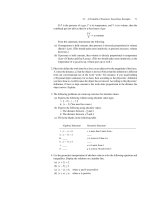
EXERCISE 11.11 Find a possible equation for the cubic function h(x) shown.
–1
1
–2
y
x
h(x)
Figure 11.17
Basic Strategy for Fitting an Equation to a Polynomial Graph
Secure the x-intercepts: If they are at x = a, x = b, and x = c, start with P(x)=
k(x − a)(x − b)(x − c).
See whether or not the sign of y changes on either side of the x-intercept.
The factor (x − a) changes sign as x increases from values less than a to those greater
than a.
If the sign changes around x = a, then the factor (x − a) must be raised to an odd
power.
If the sign of y does not change around x = a, then the factor (x − a) must be raised
to some even power.
8
If you know both the x- and y-coordinates of some point that is not a zero, use this

information to find k. If this information is unavailable, check the sign somewhere to
determine the sign of k.
8
Generally it’s wise to begin with the lowest power that has the appropriate effect. (Doing Exercise 11.10 will help you with
this.) Below are figures illustrating the effect of (x − a) versus (x − a)
3
in the neighborhood of x = a. Increasing the power of
(x − a) will flatten the graph in the immediate vicinity of x = a and make it steeper far away from x = a.
a
x
x – a
(x – a)
3
a
x
11.3 Polynomial Functions and Their Graphs 399
Take a bird’s-eye view to make sure your answer is reasonable. Look at the degree and
the leading coefficient.
REMARK This strategy is good for finding equations to fit graphs where nothing too exciting
or extravagant is happening between the zeros. It won’t help substantially in any of the cases
sketched below.
y
x
y
x
y
x
f(x)
f(x)
f(x)

Figure 11.18
PROBLEMS FOR SECTION 11.3
1. Suppose you are given a polynomial expression in both factored and nonfactored form.
When might you prefer one form over the other?
2. Suppose P(x)is a polynomial whose derivative is P

(x) = x
2
(x + 2)
3
.
(a) What degree is P(x)?
(b) What are the critical points of P(x)?
(c) Does P(x) have an absolute minimum value? If so, where is it attained? Is it
possible to find out what this minimum value is, if it exists? If yes, explain how;
if no, explain why not.
3. Let p(x ) be a polynomial of degree n. What is the maximum number of points of
inflection possible for the graph of p(x )?
4. A company is producing a single product. P(x), the profit function, gives profitasa
function of x, the number of hundreds of items produced. Suppose P(0)=−200 and
P

(x) = x
2
(x − 1)
3
.
Sketch the graph of P . Argue, using the sign of P

(x), that the graph of P intersects

the positive x-axis exactly once, i.e., for x>0,that there is one and only one break-
even point and that, if production levels are high enough, the profit will remain positive
and increase with increasing x. The following questions will help guide you.
(a) First, draw a rough sketch of the graph of P

(x). (You need not determine precisely
the position of the local minimum of P

; in other words, you need not take the
second derivative—just use what you know about the intercepts and sign of P

(x).)
(b) Draw a number line and on it record the sign of P

. Above it indicate where P is
increasing and decreasing.
(c) Now, using the information that P(0)=−200 along with the information from part
(b), make a rough sketch of P . You need not determine the positive x-intercept,
just convincingly assert that it exists.
5. Suppose P(x) with domain (−∞, ∞) is a polynomial of degree 4 whose leading
coefficient is −3. For each statement given below, determine whether the statement is
400 CHAPTER 11 A Portrait of Polynomials and Rational Functions
necessarily true, or
possibly true, possibly false, or
definitely false.
Think carefully. This is a problem concerning both logic and polynomials.
(a) lim
x→∞
P(x)=∞
(b) lim

x→−∞
P(x)=−∞
(c) P(x)has four zeros.
(d) P(x)has at least one turning point.
(e) P(x)has exactly two turning points.
(f) P(x)has four critical points.
(g) P(x)has an absolute maximum value.
(h) P(x)has an absolute minimum value.
6. Suppose P(x) is a polynomial of degree 7 whose leading coefficient is 2. For each
statement given below, determine whether the statement is
necessarily true, or
possibly true, possibly false, or
definitely false.
If you decide the statement is not necessarily true, explain your reasoning!
(a) P(x)has at least one zero and at most seven zeros.
(b) P

(x) has no zeros.
(c) P(x)has at least one point of inflection.
(d) P(x)has five points of inflection.
7. Graph f(x)=
x
4
4
+ x
3
− 5x
2
. Indicate the x-coordinates of all local extrema and all
points of inflection. What is the absolute minimum value of f ? The absolute maximum

value?
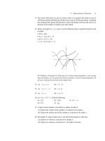
8. Find equations that could correspond to the graphs of the polynomials drawn below.
y
x
(a)
12–2
3
y
x
(b)
12–2
–3
y
x
(c)
–1
–2
(1, 2)