Calculus: An Integrated Approach to Functions and their Rates of Change, Preliminary Edition Part 43 ppsx

11.3 Polynomial Functions and Their Graphs 401
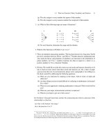
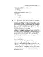
9. Find a possible equation to fit each polynomial graph below. Notice that a is a negative
number.
y
x
ab
d
c
(a)
y
x
abc
(b)
(–1, 3)
10. Find a polynomial to fit the graph below.
y
x
1
1
–3
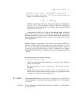
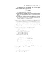
11. Each of the graphs on the following page is the graph of a polynomial P(x).For each
graph do the following.
(a) Determine whether the degree of P(x)is even or odd.
(b) Despite the fact that you have just categorized each of the polynomials as being
of either odd or even degree, none of the polynomials graphed are even functions
and none are odd functions. Explain.
(c) Determine whether the leading coefficient is positive or negative.
(d) Determine a good lower bound for the degree of the polynomial. Explain your
reasoning. (For example, the last graph on the right has one turning point, so it
must be of degree 2 or more. It is not a parabola since it has a point of inflection;
therefore we know the degree is higher than 2. It cannot be a polynomial of degree

3 because for |x| large enough, P(x)is positive. Therefore, it must be a polynomial
of degree 4 or more.)
402 CHAPTER 11 A Portrait of Polynomials and Rational Functions
P
x
(i)
P
x
(ii)
P
x
(iii)
12. (a) Suppose P(x) is a polynomial of degree 5. Which of the statements that follow
must necessarily be true? If a statement is not necessarily true, provide a coun-
terexample (an example for which the statement is false).
i. P(x) has at least one zero.
ii. P(x) has no more than four zeros.
iii. The graph of P(x) has at least one turning point.
iv. The graph of P(x) has at most four turning points.
(b) Suppose P(x) is a polynomial of degree 5 with its natural domain (−∞, ∞).If
P

(π) = 0 and P

(π) = 5, then which one of the following statements is true?
Explain your answer.
i. P has a local minimum at x = π but this local minimum is not an absolute
minimum.
ii. P has a local minimum at x = π and this local minimum may be an absolute
minimum.

iii. P has a local maximum at x = π but this local maximum is not an absolute
maximum.
iv. P has a local maximum at x = π and this local maximum may be an absolute
maximum.
13. (a) Suppose P(x) is a polynomial of degree 6. Which of the statements that follow
must necessarily be true? If a statement is not necessarily true, provide a coun-
terexample (an example for which the statement is false).
i. P(x) has at least one zero.
ii. P(x) has no more than five zeros.
iii. The graph of P(x) has at least one turning point.
iv. The graph of P(x) has at most five turning points.
(b) Suppose P(x) is a polynomial of degree 6 with its natural domain (−∞, ∞).If
P

(2)=0and P

(2) =−1, then which one of the following statements is true?
Explain your answer.
i. P has a local minimum at x = 2 but this local minimum is not an absolute
minimum.
ii. P has a local minimum at x = 2 and this local minimum may be an absolute
minimum.
iii. P has a local maximum at x = 2 but this local maximum is not an absolute
maximum.
iv. P has a local maximum at x = 2 and this local maximum may be an absolute
maximum.
11.3 Polynomial Functions and Their Graphs 403
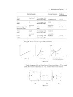
14. For each of the graphs below, all vertical and horizontal asymptotes are indicated with
dotted lines. If there are no dotted lines there are no asymptotes.
(a) Which of the following could possibly be the graph of a polynomial function? If

the graph could be the graph of a polynomial, what can you say about the degree
of the polynomial? Can you determine whether the degree is even or odd? Can you
determine an n such that the degree of the polynomial is at least n?
(b) Which could possibly be the graph of a function of the form f(x)=Cb
x
+D,
where C, b, and D are constants?
(c) For each of the remaining graphs (graphs not listed as answers to the previous two
questions), what characteristic of the graph made you rule it out?
y
x
y
x
y
x
y
x
y
x
y
x
(i) (ii) (iii)
(iv) (v) (vi)
15. The functions that follow in this exercise are not polynomials. We ask you about
their range, domain, and graphs with the goal of having you appreciate how nicely
polynomial functions behave. For each of the following functions:
(a) Determine the domain.
(b) Determine the range.
(c) Sketch a graph of the function. Do this using your knowledge of flipping, stretch-
ing, shrinking, shifting, and of graphing

1
f(x)
;check your graph with your graphing
calculator.
Your answers to parts (a) and (b) ought to agree with your answer to part (c). You
can use your answers to parts (a) and (b) to select an appropriate viewing window in
your calculator.
i. f(x)=
5
x+20
(The basic shape, before shifts and stretches,
is y = 1/x.)
ii. g(x) =−2
√
x − 100 (The basic shape, before shifts and stretches,
is y =
√
x.
iii. h(x) =
1
√
x+40
(Graph y =
√
x, shift, and then look at the
reciprocal.)
iv. j(x)=
2
(x−20)(x+30)
(Graph y = (x − 20)(x + 30), then look at

the reciprocal.)
404 CHAPTER 11 A Portrait of Polynomials and Rational Functions
Exploratory Problems for Chapter 11
Functions and Their Graphs: Tinkering with Polynomials and Rational Functions
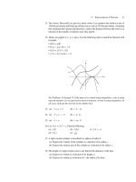
1. Find a polynomial function P(x)that fits the graph drawn below.
The x-intercepts should be at x =−2and x = 0 and the function
should have a global minimum of −6. It is not clear exactly where
this minimum is attained.
y
x
–2
–6
f(x)
Figure 11.19
The goal of this problem is to encourage you to tinker with
the equation using what you know about polynomials and their
derivatives. The first few questions below are designed to steer
you in the right direction.
(a) Is P(x) apolynomial of even degree, or of odd degree?
(b) Give a lower bound for the degree of P(x).Explain.
(c) What are the roots of P(x)?Takeafirst guess at the equation
for P(x) in factored form.
(d) What can you do (or what have you done) to make the graph
of P(x) flatten out at x = 0?
(e) Adjust your formula to assure that the minimum value of P(x)
will be −6.
Do you want to stretch vertically or do you want to shift
vertically? You don’t want to uproot the x-intercepts you have
so carefully nailed into place.
(f) Write a formula for P(x).

(g) Given your answer to the last question, determine where P(x)
takes on its minimum value.
Your answer should come from your function and be deter-
mined by analyzing its derivative; don’t simply guess by read-
ing off the graph.
The next set of problems asks you to think about rational
functions, the topic of the next section of this chapter.
Exploratory Problems for Chapter 11 405
2. Graph each function f and under it, graph its reciprocal,
1
f(x)
.
Then answer the following questions in as much generality as you
can.
(a) How is the sign of
1
f(x)
related to the sign of f ?
(b) How is the magnitude (the absolute value) of
1
f(x)
related to
the magnitude of f ?
(c) What characteristic(s) of f determines the location and type
of vertical asymptote of
1
f(x)
?
i. f(x)= x ii. f(x)= x
2

iii. f(x)= x
2
− 1iv.f(x)= x(x − 3)
3. This problem should be done with the aid of a graphing calculator
or computer. Give a very rough sketch of the graph of each of the
following. If you like, a group can get together and split up the
work, each person graphing a couple of these functions on his or
her calculator. The important thing is for you to think about the
relationships between the equations and their graphs.
(a) y =
1
x−1
(b) y =
1
(x−1)
2
(c) y =
1
x(x−1)
(d) y =
1
x
2
(x−1)
(e) y =
1
x(x−1)
2
(f) y =
1

x
2
(x−1)
2
(g) y =
x
(x−1)
(h) y =
x
2
(x−1)
Think about the relationships between these equations and their
graphs, the effect of the factors in the denominators, and the effect
of squaring certain factors. Present as many observations as you
can come up with.
406 CHAPTER 11 A Portrait of Polynomials and Rational Functions
11.4 RATIONAL FUNCTIONS AND THEIR GRAPHS
An Introduction to Rational Functions
Rational functions are functions of the form f(x)=
polynomial in x
polynomial in x
. They are a class of
functions that includes the polynomials
9
(a well-behaved family) as well as some more
unruly relatives. Rational functions can exhibit much wilder and more varied behavior
than polynomials. They may be undefined for certain values of x, and therefore may be
discontinuous. Not only may they be discontinuous, but the magnitude of f may blow
up around a point of discontinuity. In other words, it is possible that lim
x→c

|f(x)|=∞
for some finite number c. In this case, the rational function has a vertical asymptote. It
is possible that lim
x→∞
f(x)=k for some finite constant k, in which case f(x) has a
horizontal asymptote. Once you become accustomed to the behavior of rational functions
and learn the relationship between the function and the behavior of its graph, you may very
well find that rational functions are fun to work with. That alone could constitute a reason
to get to know these functions. But there are more practical reasons as well.
An economist interested in the average cost per pound of producing q pounds of a
good will divide the total cost function, C(q), by the number of pounds produced. If C(q)
is modeled by a polynomial, then
average cost per item =
C(q)
q
is a rational function.
Any time two variables are inversely proportional to one another, there is a functional
relationship of the form f(x)=k/x, a form with which we have longstanding familiarity.
Scientists observing naturally occurring phenomena have found such relationships ubiqui-
tous. For instance, chemists use the combined gas laws relating the pressure, P , temperature,
T , and volume, V ,ofagas:
PV =kT or P =
kT
V
.
Physicists have found that the gravitational attraction between two objects is inversely
proportional to the square of the distance between them. For example, a rocket on a journey
in space will be subject to the gravitational force of the earth. The acceleration due to the
gravitational attraction of the earth is given by
Gm

E
r
2
,
where G is the universal gravitational constant, m
E
is the mass of the earth, and r is the
distance from the rocket to the center of the earth. If the rocket is journeying from the earth
to the moon, then the primary forces acting on it are the gravitational forces of the earth and
the moon. The acceleration due to the gravitational attraction of the moon is given by
Gm
M
R
2
,
9
If the polynomial in the denominator is a constant, then f(x)is simply a polynomial.
11.4 Rational Functions and Their Graphs 407
where G is as above, m
M
is the mass of the moon, and R is the distance from the rocket to
the moon’s center.
Let G be the acceleration of the rocket due to the combined gravitational forces of the
earth and moon.
A =

acceleration due to
the earth’s gravity

−


acceleration due to
the moon’s gravity

.
The two terms have opposite signs because, from the perspective of the rocket, the forces
act in opposite directions. The distance between the center of the earth and the center of
the moon is roughly 240,000 miles. We’ll call this distance D. Then, when the rocket is a
distance x from the center of the earth, its distance from the center of the moon is D − x.
Earth
rocket moon
x
D-x
Figure 11.20
A(x) =
Gm
E
x
2
−
Gm
M
(D − x)
2
,or
A(x) = G

m
E
(D − x)

2
− m
M
x
2
x
2
(D − x)
2

.
A is a rational function of the rocket’s distance from the center of the earth.
Removable and Nonremovable Discontinuities and Asymptotes
The main ways in which rational functions can deviate from the behavior of polynomials
are that they can have discontinuities (removable or nonremovable) and can have vertical
and horizontal asymptotes.
10
Points of Discontinuity
A rational function f(x)will be undefined (and hence discontinuous) wherever the denom-
inator is zero.
Removable Discontinuities: A bug’s-eye view. If the denominator and the numerator of a
rational function are both zero at x = b, then the numerator and denominator have a common
factor of x − b. If these factors occur with the same multiplicity,
11
then the graph has a
pinhole at x = b. A pinhole, i.e., a situation in which lim
x→c
+
f(x)=lim
x→c

−
f(x)=L
where L is finite, but f(c)=L,isreferred to as a removable discontinuity.
10
The nonremovable discontinuities show up as vertical asymptotes.
11
What is actually required is that the multiplicity in the numerator is greater than or equal to that in the denominator. For
example, if f(x)=
(x
2
+1)x
2
x
, then f(x)=

(x
2
+ 1)x for x = 0
undefined for x = 0
and the graph of f has a pinhole at x = 0.
If g(x) =
(x
2
+1)x
x
2
, then, g(x) =

x
2

+1
x
for x = 0
undefined at x = 0
. The graph of g(x) has a vertical asymptote at x = 0.
408 CHAPTER 11 A Portrait of Polynomials and Rational Functions
y
x
y =
(x
2
+ 1)x
x
pinhole at x = 0
Figure 11.21
Vertical Asymptotes: A bird’s-eye view. If the denominator of a rational function is zero
at x = b and the numerator is nonzero, then the graph has a vertical asymptote at x = b.
12
We need a bird’s-eye view because as x approaches b, f(x) will either increase without
bound or decrease without bound. If f has a vertical asymptote at x = b, then near x = b
the graph of f will look like one of the graphs shown in Figure 11.22.
x = b
For instance,
f(x) =
1
(x–b)
2
x = b
For instance,
f(x) =

1
x–b
x = b
For instance,
f(x) =
–1
(x–b)
2
x = b
For instance,
f(x) =
–1
x–b
Figure 11.22
Simple sign information will distinguish between the four options. The base idea behind this
is just what we discussed in Chapter 7 when looking at lim
x→0
+
1
x
=∞and lim
x→0
−
1
x
=
−∞. The graph will never cross its vertical asymptotes because the function is undefined
there.
Horizontal Asymptotes: A bird’s eye-view of rational functions.
13

A horizontal asymp-
tote suppliesinformation about f as the magnitude of x increases without bound; it indicates
the behavior of the function toward the extremities of the graph in the case where these ex-
tremities look like horizontal lines. If lim
x→∞
f(x)=K for some (finite) constant K,we
say f has a horizontal asymptote at K, and similarly if lim
x→−∞
f(x)=K. Recall that
polynomials never have horizontal asymptotes, and exponential functions have one-sided
horizontal asymptotes. For any rational function f , if lim
x→∞
f(x)=K where K is finite,
then lim
x→−∞
f(x)=K as well; the horizontal asymptotes are two-sided. In order to in-
vestigate whether or not the graph of a rational function f(x)has a horizontal asymptote,
we must look at the behavior of f as x →∞and x →−∞.Forxvery large in magnitude,
any polynomial is dominated by its term of highest degree; therefore, we will break down
our investigations into cases in which we are concerned with the relative degrees of the
12
What is actually required is that b is a zero of the denominator, and if it is also a zero of the numerator, the multiplicity of
the root in the numerator is less than that in the denominator.
13
A bird’s-eye view would catch both horizontal and vertical asymptotes, but miss removable discontinuities.
11.4 Rational Functions and Their Graphs 409
numerator and the denominator of the rational function. We will use the fact that for any
positive integer n and any constant k, lim
x→∞
k

x
n
= 0.
Case I. Degree of Numerator Less Than Degree of Denominator
◆
EXAMPLE 11.11 f(x)=
x−1
2x
2
−x−3
. Calculate lim
x→∞
x−1
2x
2
−x−3
.
SOLUTION Both the numerator and the denominator of this fraction are growing without bound, but
the denominator grows much more rapidly than the numerator. (Try this out numerically on
your calculator for very large x.) For x very large in magnitude the term of highest degree
dominates any polynomial, so the numerator “looks like” x and the denominator like 2x
2
.
Therefore, from a bird’s-eye view, for x very large in magnitude f(x)looks like
x
2x
2
=
1
2x

.
lim
x→∞
1
2x
= 0.
More formally, we can get a handle on this limit by dividing the numerator and
denominator by the highest power of x occurring in the denominator:
lim
x→∞
x − 1
2x
2
− x − 3
= lim
x→∞
x
x
2
−
1
x
2
2x
2
x
2
−
x
x

2
−
3
x
2
= lim
x→∞
1
x
−
1
x
2
2 −
1
x
−
3
x
2
=
0
2
= 0.
Similarly, we can show lim
x→−∞
f(x)= 0.
◆
This argument can be generalized to show that if the degree of the numerator is less
than the degree of the denominator, then the rational function has a horizontal asymptote at

y = 0, the x-axis.
Case II. Degree of Numerator Equal to Degree of Denominator
◆
EXAMPLE 11.12 f(x)=
x
2
−1
2x
2
−x−3
. Calculate lim
x→∞
x
2
−1
2x
2
−x−3
.
SOLUTION Both the numerator and the denominator of this fraction are growing without bound, but
the denominator is growing about twice as rapidly as is the numerator. From a bird’s-eye
view, for x very large in magnitude the numerator “looks like” x
2
and the denominator like
2x
2
. Therefore, for x very large in magnitude f(x)looks like
x
2
2x

2
=
1
2
. Again, you can test
this out numerically on your calculator for very large x.
More formally, we can get a handle on this limit by dividing the numerator and
denominator by the highest power of x occurring in the denominator:
lim
x→∞
x
2
− 1
2x
2
− x − 3
= lim
x→∞
x
2
x
2
−
1
x
2
2x
2
x
2

−
x
x
2
−
3
x
2
= lim
x→∞
1 −
1
x
2
2 −
1
x
−
3
x
2
=
1
2
.
Similarly, we can show lim
x→−∞
f(x)=
1
2

.
◆
This argument can be generalized to show that if the degree of the numerator is equal
to the degree of the denominator, then the rational function has a horizontal asymptote at
y =
leading coefficient of numerator
leading coefficient of denominator
.
Case III. Degree of Numerator Greater Than Degree of Denominator
◆
EXAMPLE 11.13 f(x)=
x
3
−1
2x
2
−x−3
. Calculate lim
x→∞
x
3
−1
2x
2
−x−3
.
410 CHAPTER 11 A Portrait of Polynomials and Rational Functions
SOLUTION Both the numerator and the denominator of this fraction are growing without bound, but
the numerator is growing much more rapidly than the denominator. From a bird’s-eye view,
for x very large in magnitude the numerator looks like x

3
and the denominator like 2x
2
.
Therefore, for x very large in magnitude f(x)looks like
x
3
2x
2
=
x
2
.Asx→∞,
x
2
→∞.
More formally, we can get a handle on this limit by dividing the numerator and
denominator by the highest power of x occurring in the denominator:
lim
x→∞
x
3
− 1
2x
2
− x − 3
= lim
x→∞
x
3

x
2
−
1
x
2
2x
2
x
2
−
x
x
2
−
3
x
2
= lim
x→∞
x −
1
x
2
2 −
1
x
−
3
x

2
= lim
x→∞
x =∞.
Wecan show lim
x→−∞
f(x)=lim
x→−∞
x =−∞.
◆
This argument can be generalized to show that if the degree of the numerator is greater
than the degree of the denominator, then the rational function has no horizontal asymptote.
Graphs from Equations/Equations from Graphs
A rational function may be discontinuous. At a point of discontinuity the function can
change sign without passing through zero. If a function is discontinous its derivative will
be discontinuous as well. (Recall that differentiability guarantees continuity, and therefore
discontinuity guarantees a lack of differentiability.) Therefore the derivative can change sign
without passing through zero and the function can change from increasing to decreasing or
vice versa without having a horizontal tangent line.
Graphing a Rational Function f(x)=
polynomial in x
polynomial in x
Simplify, if possible, and look for pinholes. Factor the numerator and the denominator;
some information is easiest to get when the expression is factored. If there is a common
factor in the numerator and denominator, cancel with care. If the common factor is (x − c),
then the function is undefined at c, so its graph has a pinhole or a vertical asymptote at c.
f(x)=
(x+1)(x+2)
(x+1)(x+3)
=

(x+2)
(x+3)
for x =−1. f(x)is undefined when x =−1.
The graph has a pinhole at x =−1.
f(x)=
(x+1)
(x+1)
2
=
1
x+1
for x =−1. f(x)is undefined when x =−1.
The graph has a vertical asymptote at x =−1.
f(x)=
(x
2
+1)(x+2)
(x
2
+1)(x+3)
=
(x+2)
(x+3)
The graph has no pinholes (x
2
+ 1) = 0.
1. Identify all vertical asymptotes. Where is the denominator of the simplified expres-
sion zero?
f(x)will be undefined at a vertical asymptote and nearby |f(x)|→∞.