Calculus: An Integrated Approach to Functions and their Rates of Change, Preliminary Edition Part 52 pdf

15.1 An Interesting Limit 491
Let’s return to Example 15.1. Recall that we have deposited $10,000 into a bank with a
nominal annual interest rate of 100% and left it for one year. If the interest were compounded
n times a year we would have $10,000(1 +
1
n
)
n
. The question is whether (1 +
1
n
)
n
increases
without bound or approaches some limiting value. (When looked at in this context, it seems
unreasonable that the limit would be 1.) Let’s experiment by returning to the numerical
approach suggested by Example 15.1 and evaluating (1 +
1
n
)
n
for large n. The largest value
we looked at in Example 15.1 was n = 525,600. Below are the results of evaluating (1 +
1
n
)
n
for various values of n using a TI-83. All the digits displayed by this calculator are recorded
here.
For n = 525,600, the TI-83 gives 2.718279215.
For n = 1,000,000, the TI-83 gives 2.718280469.

For n = 10
10
, the TI-83 gives 2.718281828.
For n = 10
15
, the TI-83 gives 1.
What are we to make of this? For starters, look at the very last result. Do you honestly
think that (1 +
1
10
15
)
10
15
= 1? No. The result must be larger than 1. As n increases, (1 +
1
n
)
n
increases; we know this from the context of the problem. What in fact is happening is that
the calculator has treated (1 +
1
10
15
) as 1 and then computed 1
10
15
and arrived at 1. Therefore,
when considering the numerical results from the calculator, we need to disregard this one. If
we evaluate (1 +

1
n
)
n
for n larger than 10
10
, the TI-83 will keep giving us 2.718281828 until
n gets so large that the TI-83 throws up its little calculator hands and gives us the number 1.
The results of our numerical investigations might lead you to wonder whether the number
2.718281828 has some significance. Where have you seen this number before? If you make
your calculator display (to the best of its ability) the number e, it will match up, decimal for
decimal, with 2.718281828.
4
This might lead you to conjecture that lim
n→∞
(1 +
1
n
)
n
= e.
What Happens to the Limit as n Grows Without Bound?
Does the Limit Equal e?
Looking at numerical data and conjecturing that lim
n→∞
(1 +
1
n
)
n

= e is great, but if we
want to verify this conjecture
5
we cannot simply try to match up decimal places. There are
two logical difficulties. First of all, e is an irrational number; e cannot be written as a finite
decimal or as an infinite repeating one, so we cannot ever hope to match all the decimal
places for e. Second, and even more fundamental, is the question of where all of these
decimal places for e are coming from to begin with. We have simply defined e to be the
number “a” such that the derivative of the function a
x
is a
x
.
6
We have to rely exclusively on
4
If you get hold of a few more digits for e, you’ll get 2.718281828459 eis an irrational number; its decimal expansion
is nonrepeating.
5
We will show lim
x→∞
(1 +
1
x
)
x
= e and then conclude that lim
n→∞
(1 +
1

n
)
n
= e. We must be careful. If lim
x→∞
f(x)=L
then lim
n→∞
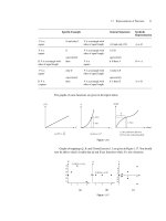
f (n) = L, but the converse is not necessarily true. If lim
n→∞
f (n) = L it is possible that lim
x→∞
f(x)=L.See
the figure below.
1–12–23
x
y
6
The Swiss mathematician Leonhard Euler, who first introduced the number e in the mid-1700s, in fact defined e to be the
limit in question (although a rigorous foundation for limits was not laid down until the 1800s). In this text we have not followed
the actual historical development and must now show that e as we defined it is the same e that Euler defined.
492 CHAPTER 15 Take It to the Limit
this definition of e. While the calculator has been instrumental in suggesting the conjecture,
it has no role in actually proving it.
7
Knowing that the derivative of e
x
is e
x
, we concluded, after some work, that the

derivative of its inverse function ln x is 1/x; this information will turn out to be useful
in verifying our conjecture. If we can show lim
x→∞

1 +
1
x

x
= e we can conclude that
lim
n→∞

1 +
1
n

n
= e.
Is lim
x→∞
(1 +
1
x
)
x
Really e?
Let’s use the longstanding tactic of naming what we are looking for. (What follows is valid
if we assume this limit exists and is finite.)
Let B = lim

x→∞

1 +
1
x

x
.
We have a variable in the exponent; we’d like to “bring it down” in order to make the
expression on the right more tractable, so we’ll take the natural logarithm of both sides of
the equation:
ln B = ln

lim
x→∞

1 +
1
x

x

.
Because the logarithm is a continuous function, this is equivalent to writing
8
ln B = lim
x→∞

ln


1 +
1
x

x

= lim
x→∞
x ln

1 +
1
x

.
As x →∞we have the product of two numbers, one of which is going toward zero
(because ln 1 = 0), and the other which is growing without bound.
9
ln(1 +
1
x
) is approaching
ln 1 = 0, but it is being multiplied by x, which is approaching ∞. It is still hard to decipher
what is going on. Our area of expertise is more along the lines of taking the limit as something
tends toward zero, and this may tie in with our defining characteristic of e. Let’s try a
substitution in hopes of figuring out this limit. Substitution is a tool for transforming the
unfamiliar into the familiar.
Let h =
1
x

.Asx→∞,h→0.
With this substitution, lim
x→∞
x ln(1 +
1
x
) becomes lim
h→0
1
h
ln(1 + h) = lim
h→0
ln(1+h)
h
.
ln B = lim
h→0
ln(1 + h)
h
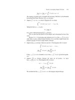
This latter limit is easier to evaluate. In fact, you may recognize that it is the definition
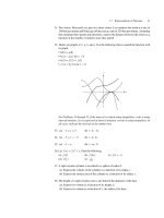
of the derivative of ln x at x = 1. Verify, using Figure 15.3, that the slope of the secant line
7
At this point, we don’t know how the calculator has arrived at its decimal expansion of e. Numerically all we have shown is
that e lies between 2.7 and 2.8. If we can prove our conjecture, then we have a way of numerically approximating e.
8
If f is a continuous function, then f(lim
x→a
g(x)) = lim
x→a
f(g(x)).This is limit principle (4).

9
Here’s another “indeterminate form”: ∞·0.On the one hand, any finite number multiplied by zero is zero. On the other
hand, if a number is growing without bound and we multiply it by any positive number, the product ought to grow without bound.
(Of course, the second factor is not identically zero; it is just tending toward zero. Neither is the first factor “∞”; it is just growing
without bound.) Again, our gut reaction to the problem pulls us in two different directions and the result churns the stomach.
15.1 An Interesting Limit 493
through (1, 0) and (1 + h,ln(1+h)) is
ln(1 + h) − ln 1
(1 + h) − 1
=
ln(1 + h)
h
.
x
y
y = ln x
1
1 + h
(1 + h, ln(1 + h))
Figure 15.3
So lim
h→0
ln(1 + h)
h
=
d
dx
(ln x)





x=1
.
The derivative of ln x is
1
x
, and evaluating at x = 1 gives 1. Therefore, ln B = 1. We were
looking for B, not ln B; exponentiating shows that B = e
1
= e. Eureka!
lim
x→∞

1 +
1
x

x
= e
Not only have we gained a whole new perspective on e, but we now have a method of
approximating e numerically.
Having computed lim
x→∞
(1 +
1
x
)
x
= e, we can compute variations on this limit.

◆
EXAMPLE 15.4 Show that for any constant r, lim
n→∞
(1 +
r
n
)
n
= e
r
.
SOLUTION To evaluate this limit we will use the technique employed so successfully above; we
will rename our variables. (Changing variables is a standard mathematical technique for
converting something that looks a bit unfamiliar to something well known and having
familiar structure.) We would like to replace
r
n
by
1
m
so we can utilize our previous result. If
1
m
=
r
n
, then mr = n,som=
n
r
. Therefore, we use the substitution m =

n
r
. We can assume
that r = 0, because the case r = 0 can be easily handled independently.
As n →∞, m=
n
r
→∞as well, because r is a constant.
Thus,
lim
n→∞

1 +
r
n

n
= lim
m→∞

1 +
1
m

mr
= lim
m→∞

1 +
1

m

m

r
.
But r is a constant, so this is equivalent to
10
10
We’ re using limit principle (4) again. If f is continuous, then lim
x→a
f(g(x))=f
(
lim
x→a
g(x)
)
.
494 CHAPTER 15 Take It to the Limit

lim
m→∞

1 +
1
m

m

r

= e
r
.
We conclude that
lim
n→∞

1 +
r
n

n
= e
r
.
◆
◆
EXAMPLE 15.5 Find lim
n→∞
(1 +
3
n
)
4n
using the result of Example 15.4.
SOLUTION CAUTION This limit business is subtle. We don’t want to ad lib. Instead, we need to use
exactly the results we have worked so hard to get.
lim
n→∞


1 +
3
n

4n
= lim
n→∞

1 +
3
n

n

4
= [e
3
]
4
= e
12
◆
Implications of the Fact that lim
n→∞
(1 +
r
n
)
n
= e

r
Recall: If you put $M
0
in a bank account with nominal annual interest rate r compounded
n times per year, then M(t), the amount of money in the account after t years, is given by
M(t) = M
0

1 +
r
n

nt
.
If we let the number of compounding periods increase without bound, we obtain
M(t) = M
0
lim
n→∞

1 +
r
n

nt
= M
0
lim
n→∞


1 +
r
n

n

t
.
Having shown that lim
n→∞

1 +
r
n

n
= e
r
, we obtain M(t) = M
0
[e
r
]
t
= M
0
e
rt
. Therefore,
if a bank with nominal annual interest rate r compounds interest continuously,

11
then the
money grows according to
M(t) = M
0
e
rt
.
EXERCISE 15.2 You plan to deposit a fixed sum of money into one of two bank accounts and leave it there
for several years. Which is a better choice of accounts, an account with a nominal interest
11
Do banks really do this? Certainly some banks compute interest on savings accounts every day. If the nominal annual interest
rate is 5% and interest is compounded daily, then
M(t) = M
0

1 +
0.05
365

365t
≈ M
0
(1.051267)
t
.
If we modeled this situation using continuous compounding, we would have
M(t) = M
0
e

0.05t
≈ M
0
(1.051271)
t
.
Depending on the situation, the latter model may be quite reasonable and simpler to use. (Even using the equation M(t) =
M
0

1 +
0.05
365

365t
distorts reality a bit, because in reality if interest is compounded at the end of each day, M(t) ought to be
a step function with a point of discontinuity each time interest is computed, and yet this function is continuous.)
15.1 An Interesting Limit 495
rate of 6% per year compounded monthly or an account with a nominal interest rate of 5
1
2
%
compounded continuously?
PROBLEMS FOR SECTION 15.1
1. Suppose you put $100,000 in a bank account with 6% interest and leave it for one year.
How much money will there be in the account if the interest is compounded
(a) annually? (b) monthly? (c) daily? (d) hourly?
2. In 1996, inflation in Russia was 22%. This was a decline from the 131% inflation rate in
1995 and the 2600% inflation rate in 1994. By contrast, the inflation rate in the United
States in 1996 was about 3%. (Boston Globe, November 2, 1996.)

Compute the amount of time it would take for prices to double under each of the four
inflation rates listed.
3. A Boston Globe article on January 1, 1997, said that the best stock of 1996 was
Information Analysis, Incorporated, which closed the year at a price of $63 per share,
an increase of 1525% during the year. The worst stock of 1996 was Mobilemedia
Corporation, which closed the year at $7/16 per share, a decrease of 97.6%.
What was the price of each of these stocks at the beginning of the year?
4. Compute the following limits. In each case stop to think of a strategy, and use whatever
strategy seems simplest to you. For several of these limits there are different approaches.
(a) lim
x→3
3
x−3
(b) lim
x→3
3
(x−3)
2
(c) lim
x→∞
(1 −
1
3x
)
7x
(d) lim
t→0
+
(1 − 2t)
1/t

5. Evaluate the following limits.
(a) lim
x→∞
e
−x
x
2
(b) lim
x→∞
x
3
e
−3x
6. Suppose you invest $10,000 in an account with a nominal annual interest rate of 5%.
How much money will you have 10 years later if the interest is compounded
(a) quarterly? (b) daily? (c) continuously?
7. (a) A certain amount of money is put in an account with a fixed nominal annual interest
rate, and interest is compounded continuously. If 70 years later the money in the
account has doubled, what is the nominal annual interest rate?
(b) Answer the same question if the interest is compounded only once a year.
8. (a) Kevin has deposited money in a bank account that compounds interest quarterly.
If the nominal interest rate is 5%, what is the effective interest rate?
(b) Ama has deposited money in a bank account that compounds interest quarterly. If
the effective interest rate is 5% per year, what is the nominal rate of interest?
9. Suppose that a person invests $10,000 in a venture that pays interest at a nominal rate of
8% per year compounded quarterly for the first 5 years and 3% per year compounded
quarterly for the next 5 years.
496 CHAPTER 15 Take It to the Limit
(a) How much does the $10,000 grow to after 10 years?
(b) Suppose there were another investment option that paid interest quarterly at a

constant interest rate r. What would r have to be for the two plans to be equivalent,
ignoring taxes?
(c) If an investment scheme paid 3% interest compounded quarterly for the first 5 years
and 8% interest compounded quarterly for the next 5 years, would it be better than,
worse than, or equivalent to the first scheme?
10. Evaluate the following. Substitution may be helpful; these problems are variations on
the theme lim
n→∞

1 +
r
n

n
.
(a) lim
x→0
+
(1 + x)
1/x
(b) lim
w→∞

w + 2
w

w
(c) lim
x→∞


x − 1
x

2n
(d) lim
n→∞

n
n + 1

n
(e) lim
x→0
+
(1 + 2x)
3/(2x)
11. Suppose you put $6000 in a bank account at 5% (nominal) annual interest compounded
continuously.
(a) How much money do you have at the end of 7 years?
(b) How much money do you have at the end of t years?
(c) What is the instantaneous rate of change of money in the account with respect to
time? (Find
dM
dt
.)
(d) True or False:
dM
dt
= 0.05M. Explain your reasoning!
(e) Write your answer to part (b) in the form M = Ca

t
and use your calculator to
approximate the value of “a” numerically.
(f) Each year, by what percent does your money grow? (This is called the effective
annual yield and, if interest is compounded more than once a year, it is always
bigger than the nominal annual interest rate.)
12. Evaluate the following limits. Keep in mind that limit calculations can be subtle—don’t
ad lib, but instead keep the limits we looked at firmly in your mind and use substitution
in order to make the transfer to the problems here. You can determine whether or not
your answer is in the ballpark by using your calculator.
(a) lim
x→∞
(1 +
1
x
)
x
(b) lim
s→∞
(1 +
1
s
)
3s
(c) lim
r→∞
(1 +
0.3
r
)

r
(d) lim
w→∞
(1 + 2w
−1
)
w
(e) lim
w→∞
(1 + (2w)
−1
)
w
13. Which is a better deal, an account offering 4% annual interest compounded continu-
ously or an account offering 4.2% interest compounded annually? What is the effective
annual yield of the former account?
14. If M(t) = M
0
e
rt
, find
dM
dt
and show that
dM
dt
= rM.
(
dM
dt

= rM is called a differential equation because it is an equation with a derivative
in it. You have just shown that M(t) = M
0
e
rt
is a solution to this differential equation.)
15.2 Introducing Differential Equations 497
15.2 INTRODUCING DIFFERENTIAL EQUATIONS
We have been characterizing exponential functions in two ways: If a quantity Q = Q(t)
grows (or decays) exponentially, then we have said either
i. Q can be written in the form Q(t) = Cb
t
, where C and b are constants; or
ii. Q changes at a rate proportional to itself:
dQ
dt
= kQ for some constant k.
The first statement gives an explicit formula for the amount, the second gives the rate of
change. Let’s express the statements in a form that makes their equivalence more transparent.
In doing so we’ll sidle up to the subject of differential equations, equations involving a rate
(or rates) of change.
REMARK In the statements above we write Q and Q(t) interchangeably, using the latter to
emphasize that Q is a function of time.
We know that statement (i) implies statement (ii); if Q(t) = Cb
t
, then
dQ
dt
= C · ln b · b
t

= ln b · Cb
t
= ln b · Q(t).
The constant “k” in
dQ
dt
= kQ is equal to ln b.
For a more aesthetically pleasing result, instead of writing Q(t) as Cb
t
, we can replace
b by e
k
and write Q(t) = Ce
kt
.Now
dQ
dt
= ln e
k
· Q = kQ.
We can rewrite statements (i) and (ii) as follows. If a quantity Q = Q(t) grows (or
decays) exponentially, then there is a constant k (k>0for growth, k<0for decay) such
that
i. Q(t) = Ce
kt
and
ii.
dQ
dt
= kQ.

Let’s put this in the framework of a bank account. If money in a bank account is growing
at a nominal rate of 10% per year compounded continuously, then the instantaneous rate of
change of money in the account is 10% of the amount in the account.

(i) M(t) = M
0
e
0.1t
(ii)
dM
dt
= 0.1M
Equation (ii) really captures the situation in a simple way. The rate of change of the
amount of money is 10% of the amount of money.
Frequently scientists have knowledge about the rate of change of a quantity and from
this (and one piece of data about amount—like the initial amount) they try to find an amount
equation. If you read scientific journals, you will find that the form Q(t) = Ce
kt
is often
used to describe exponential growth or decay. If the scientist began with an equation of the
form
dQ
dt
= kQ describing the rate of change of the quantity in question, then that is the
most natural form for the amount equation. The equation
dQ
dt
= kQ is called a differential
498 CHAPTER 15 Take It to the Limit
equation. It is a differential equation that arises in many different disciplines, so we will

take this opportunity to look at it more closely.
Differential Equations and Their Solutions
Definition
An equation that contains a derivative (or derivatives) is called a differential
equation.
Some examples of differential equations are:
dy
dx
=3,
dy
dt
=2t, and
dy
dt
=y.
A function is a solution to a differential equation if it satisfies the differential equation; by
this we mean that when the function and its derivative(s) are substituted in the appropriate
places in the differential equation, the two sides of the equation are equal. A differential
equation will actually have a whole family of solutions. A solution whose parameters have
been determined is called a particular solution.
For example, the differential equation
dM
dt
=0.1 has solutions M(t) =Ce
0.1t
, where C
can be any constant at all. M(t) =Ce
0.1t
gives a family of solutions. In fact, it can be proven
that this is the general solution to the differential equation, meaning that any solution to

the differential equation can be written in this form. M(t) =350e
0.1t
is a particular solution
to the differential equation.
Checking a solution to a differential equation is analogous to checking a solution to
an algebraic equation in that if we are solving for y, then to check we must replace all
occurrences of y (whether in the form y, y

,ory

) by the proposed solution.
For example, to check whether y =−1isasolution to the algebraic equation y
2
− 3 =
2y, we replace all occurrences of y by −1 (whether in the form y or y
2
or ).Wesimply
evaluate both sides of the equation at y =−1.
(−1)
2
− 3
?
=
2(−1)
1 − 3
?
=
−2
−2 =−2
√

y=−1isasolution.
Analogously, to check whether y(t) =e
−t
is a solution to the differential equation
d
2
y
dt
2
−3y =2
dy
dt
, we evaluate both sides of the equation with y = e
−t
.
d
2
dt
2
[e
−t
] −3[e
−t
]
?
=
2
d
dt
[e

−t
]
d
dt
[−e
−t
] −3e
−t
?
=
−2e
−t
e
−t
−3e
−t
?
=
−2e
−t
−2e
−t
=−2e
−t
√
y=e
−t
is a solution.
15.2 Introducing Differential Equations 499
◆

EXAMPLE 15.6 Look for a solution to each of the differential equations given:
(a)
dy
dx
=3 (b)
dy
dt
=2t (c)
dy
dt
=y.
Then look for a family of solutions. Verify that this family of functions actually solves the
differential equation.
SOLUTION
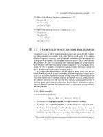
(a)
dy
dx
=3. We’re looking for a function y(x) whose derivative is 3.
y = 3x will do. It’s a line with slope 3.
y = 3x + 2 will work as well.
More generally, we have y = 3x +C for any constant C.
y
x
Figure 15.4 A family of lines with slope 3
Check: The differential equation is
dy
dx
=3. Is y = 3x + C a solution? Replace y by
3x + C and see if the two sides are equal.
d

dx
[3x + C]
?
=
3
3 = 3
√
(b)
dy
dt
=2t.We’re looking for a function y(t) whose derivative is 2t.
y = t
2
will do. Its derivative is 2t .
More generally, we can use y = t
2
+ C for any constant C.
y
x
Figure 15.5 A family of parabolas with slope 2t
500 CHAPTER 15 Take It to the Limit
Check: The differential equation is
dy
dt
=2t.Isy=t
2
+Casolution? Replace y by
t
2
+ C and see if both sides are equal.

d
dt
[t
2
+C]
?
=
2t
2t =2t
√
(c)
dy
dt
=y.We’re looking for a function y(t) whose derivative is itself. We know of one
function whose derivative is itself: e
x
. But we want a function of t,soy(t) =e
t
.
Thinking back to what we were doing right before introducing the term “differen-
tial equation,” we see that more generally y = Ce
t
for any constant C.
Check: The differential equation is
dy
dx
=y.Isy=Ce
t
a solution? Replace y by Ce
t

and see if both sides are equal.
d
dt
[Ce
t
]
?
=
Ce
t
Ce
t
=Ce
t
√
y
x
y = Ce
t
for C > 0
y = Ce
t
for C < 0
Figure 15.6
◆
Suppose that, carried away by the success of adding C in parts (a) and (b), we thought
that y = e
t
+ C might be a solution. Let’s check it.
Check:

dy
dt
=y.Isy=e
t
+Casolution? Replace y by e
t
+ C and see if both sides are
equal.
d
dt
[e
t
+C]
?
=
e
t
+C
e
t
?
=
e
t
+C No (unless C = 0).
So y = e
t
+ C is not a solution to the differential equation.
We have verified that if Q(t) = Ce
kt

, then
dQ
dt
=kQ; we know that the family of
functions Q(t) = Ce
kt
is a solution to the differential equation
dQ
dt
=kQ. In fact, any
solution must be of this form, so we refer to Q(t) =Ce
kt
as the general solution to the
differential equation.
REMARK When we study differential equations in greater depth we will see that if
dy
dt
=
f(t),then, having found one solution, we can find the general solution by adding a constant
C, whereas if
dy
dt
=f(y),this is not the case. See if you can make sense of this graphically.