Calculus: An Integrated Approach to Functions and their Rates of Change, Preliminary Edition Part 74 pps

PART
VIII
Integration: An Introduction
22
CHAPTER
Net Change in Amount and
Area: Introducing the
Definite Integral
22.1 FINDING NET CHANGE IN AMOUNT: PHYSICAL AND
GRAPHICAL INTERPLAY
Introduction
The derivative allows us to answer two related problems.
How do we calculate the instantaneous rate of change of a quantity?
How do we calculate the slope of the line tangent to a curve at a point?
The physical and graphical questions are intertwined; the slope of the graph of an “amount”
function can be interpreted as the instantaneous rate of change of the function.
Given an “amount” function, we can derive a “rate” function; we now shift our
viewpoint and investigate the problem of how to recover an “amount” function when given a
“rate” function.
1
If we know the rate of change of a quantity, how can we find the net change
in the quantity over a certain time period? Suppose, for example, that we know an object’s
velocity over a specified time interval. Then we ought to be able to use that information to
1
We did this when we looked at projectile motion in Section 20.7.
711
712 CHAPTER 22 Net Change in Amount and Area: Introducing the Definite Integral
determine the object’s net change in position during that time. To figure out how to do this
we begin by looking at some simple examples where the rate of change is constant and then
apply what we learn to cases where the rate of change is not constant.
Let’s clarify what is meant by net change. If you take two steps forward and one step

back, your net change in position is one step forward. If, over the course of a day, the stock
market falls 100 points and then gains 40 points, the net change for the day is −60 points.
We now prepare to tackle the following two questions.
Given a rate function, how do we calculate the net change in amount?
How do we calculate the area under the graph of a function?
In this chapter we aim to convince you that the physical and graphical questions are closely
related. We’ll approach the questions using the strategy that served us so well in developing
the derivative: the method of successive approximation followed by a limiting process.
Calculating Net Change When Rate of Change Is Constant
◆
EXAMPLE 22.1 Suppose that a moose is strolling along at a constant velocity. The distance she travels can
be calculated by the familiar formula distance = (rate) · (time).
If the moose moves at 4 miles per hour between 1:15 p.m. and 1:30 p.m., the distance
she has traveled (or her net change in position) is
4
miles
hour
·
1
4
hours = 1 mile,
where the units cancel to give us an answer in the units we expect.
More generally, let s(t) be the position of an object at time t and suppose that its
velocity,
ds
dt
,isconstant between times t = a and t = b.
net change in position = (rate of change of position) · (time elapsed)
s =
ds

dt
· t
t denotes the change in time, t = (b − a), and s = s(b) − s(a).
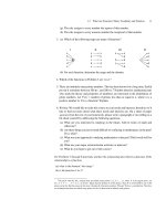
We can represent the net change in position graphically.
∆t
t
ab
ds
dt
Figure 22.1
When velocity is constant, net change in position is calculated by multiplying rate of
change,
ds
dt
, by time; geometrically, this corresponds to the area of the shaded rectangle in
Figure 22.1.
◆
◆
EXAMPLE 22.2 Let W(t) be the amount of water in a swimming pool as a function of time, where time is
measured in hours. Suppose the pool is being filled at a constant rate of
dW
dt
gallons per hour
22.1 Finding Net Change in Amount: Physical and Graphical Interplay 713
between noon and 12:30 p.m. In that half-hour,
the net change in amount of water = rate at which water is entering · (time elapsed)
W =
dW
dt
· t,

where t is one-half of an hour.
Graphically, this net change can be represented as the area of the rectangle shaded in
Figure 22.2.
t
dW
dt
noon 12:30
Figure 22.2
◆
◆
EXAMPLE 22.3 Let C(x) be the cost (in dollars) of producing x grams of feta cheese. Suppose that for each
additional gram produced the cost increases by a constant amount;
dC
dx
is constant.
2
Then,
the net change
in production cost
=
rate of change
of cost per gram
·
change in number
of grams produced
C =
dC
dx
· x
Notice that the independent variable (in this case x, the number of grams of cheese produced)

does not have to represent time.
x
dC
dx
∆ x
ab
Figure 22.3
◆
◆
EXAMPLE 22.4 On a certain day, the temperature in Kathmandu decreases at a constant rate of two degrees
per hour from 6:00 p.m. to 10:00 p.m. If we let T (t) be the temperature at time t , we can
write the following.
net change in temperature = rate of change of temperature · (time elapsed)
T =
dT
dt
· t
T = (−2)
degrees
hour
· (10 − 6) hours
=−8degrees
2
Students of economics will recognize this as marginal cost.
714 CHAPTER 22 Net Change in Amount and Area: Introducing the Definite Integral
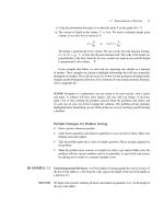
When we represent this geometrically, we have a rectangle under the t-axis. We’d like
to convey the information that T is negative by attaching a sign to the area. The net change
in temperature is negative because the temperature is decreasing;
dT
dt

is negative. We can
say that the “height” of the rectangle is −2 (since it lies below the t-axis) and assign the
rectangle a signed area of −8.
t
dT
dt
–2
610
Figure 22.4
When using areas to represent net changes, we will use the idea of “signed area”—areas
are positive or negative, depending on whether the region lies above or below the horizontal
axis.
To illustrate further how signed area is used, suppose that we also know that the
temperature in Kathmandu on this particular day increased at a rate of 1.5 degrees per hour
between 3:00 p.m. and 6:00 p.m.
T from 3:00 p.m. to 6:00 p.m. = 1.5
degrees
hour
· (6–3) hours
= 4.5 degrees
Putting the two time periods together gives a net change of 4.5
◦
+ (−8
◦
) =−3.5
◦
between
3:00 p.m. and 10:00 p.m. Graphically, this is represented by one rectangle above the t -axis
(when
dT

dt
is positive) and one rectangle below the t-axis (when
dT
dt
is negative).
t
dT
dt
63
10
Figure 22.5
REMARK: Although we know that the temperature dropped 3.5 degrees between 3:00 p.m.
and 10:00 p.m., we have no idea of what the temperature actually was at any time. We need
to know one specific data point for the function T (t) before we can determine any actual
values of T . For example, if we knew that at 3:00 p.m. the temperature was 55 degrees, then
we would know that T(10) = 55 − 3.5 = 51.5 degrees. In fact, we could calculate T (t) for
any time between 3:00 p.m. and 10:00 p.m. On the other hand, if the temperature at 3:00 p.m.
was 40 degrees, then T(10) = 40 − 3.5 = 36.5.
◆
As illustrated by the preceding examples, finding a quantity’s net change is straightfor-
ward provided that its rate of change is constant. However, the rate of change often is not
constant. How can we approach these situations?
22.1 Finding Net Change in Amount: Physical and Graphical Interplay 715
Approximating Net Change When Rate of Change is Not Constant
◆
EXAMPLE 22.5a Suppose that a cheetah’s velocity is given by v(t) = 2t + 5 meters per second on the interval
[1, 4]. Approximate its net change in position over this interval by giving upper and lower
bounds that differ by less than 0.1 meter.
(4, 13)
(1, 7)

v(t)
t
Figure 22.6
SOLUTION The problem we face is analogous to the one confronting us when we first set out to find
the slope of a curve. At that time, we knew how to find the slope of a straight line, but not
the slope of a curve, so we approximated the slope of a curve at x = a by the slope of a
secant line through points (a, f(a))and (a + x, f(a+x)). To get successively better
approximations, we repeatedly shortened the interval x. Then, to obtain an exact value
for the slope at x = a, we evaluated the limit as x approached zero.
To tackle the present problem, we will follow a similar procedure, that of successive
approximations. If r(t) is a nonconstant rate of change on an interval [a, b], we divide the
interval into smaller subintervals estimate the net change within each of those subintervals,
and sum to find the accumulated change. On each of these subintervals we approximate r(t)
by a constant rate of change.
The Method of Successive Approximations
Take One. The function v(t) is increasing throughout the interval [1, 4], so the velocity is
at least v(1) = 7 m/sec and at most v(4) = 13 m/sec.
7 ≤ v(t) ≤ 13, for all t in the interval [1, 4].
If the cheetah were moving at a constant rate, then its net change in position would be given
by (rate) · (time); therefore we know the following.
(7m/sec) · (3 sec) ≤ net change in position ≤ (13 m/sec)(3 sec)
21 meters ≤ net change in position ≤ 39 meters
Therefore, the cheetah moved between 21 and 39 meters.
v(t)
t
7
13
14
Figure 22.7
How can we improve on these bounds?

Take Two. To get a better approximation, let’s divide the interval [1, 4] into smaller
subintervals and approximate the rate of change by a constant function on each subinterval.
716 CHAPTER 22 Net Change in Amount and Area: Introducing the Definite Integral
For the sake of convenience, let’s divide the interval into three subintervals of equal width,
[1, 2], [2, 3], and [3, 4], and call the width of each subinterval t.
3
The table below shows
the velocity of the cheetah at the endpoints of each of these subintervals.
1234
∆t∆t∆t
t 123 4
v(t) 791113
v(t)
t
7
13
1234
Figure 22.8
Because the velocity is increasing on the interval [1, 4], the velocity is least at the
beginning of each subinterval (i.e., at the left endpoint) and greatest at the end of each
subinterval (the right endpoint). During the time interval [1, 2] the velocity is greater than
or equal to v(1) = 7 m/sec and less than or equal to v(2) = 9 m/sec. Again using the fact
that if rate is constant, (rate) · (time) = net change, we deduce the following.
v(1) · (1 sec) = (7 m/sec) · (1 sec) = 7misalower bound for the distance traveled in
the interval [1, 2]
v(2) · (1 sec) = (9 m/sec) · (1 sec) = 9misanupper bound for the distance traveled
in the interval [1, 2]
We can refer to the lower bounds and upper bounds as “underestimates,” and “overesti-
mates,” respectively.
We use the same method to get lower and upper bounds for the distance the object

travels in each of the other subintervals. Adding together the lower bounds for the three
subintervals will give us a lower bound for the net change in the cheetah’s position over the
entire interval [1, 4]; similarly, summing the upper bounds for the subintervals will give an
upper bound for the whole interval.
lower bound for the net
change in position on [1, 4]
v(1) · 1 + v(2) · 1 + v(3) · 1 = 7 · 1 + 9 · 1 + 11 · 1 =
27 meters
upper bound for the net
change in position on [1, 4]
v(2) · 1 + v(3) · 1 + v(4) · 1 = 9 · 1 + 11 · 1 + 13 · 1 =
33 meters
The net change in the cheetah’s position on [1, 4] is more than 27 meters and less than
33 meters.
3
Here t = 1, but we will soon subdivide further, and as we do so t will shrink.
22.1 Finding Net Change in Amount: Physical and Graphical Interplay 717
v(t)
t
7
9
11
1234
lower bound (left-hand sum)
v(t)
t
9
11
13
1234

upper bound (right-hand sum)
Figure 22.9
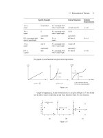
When we approximate the value of a function over each subinterval by using the value
of the function at the left endpoint of each subinterval, then multiply by the length of the
subinterval and sum the results, we call the sum a left-hand sum. It is denoted by L
n
, where
n denotes the number of subintervals. When we use the right endpoints of each subinterval,
we call the sum a right-hand sum and denote it by R
n
.
In this example, because the function v(t) is increasing, the left-hand sum will be a
lower bound and the right-hand sum will be an upper bound. In the graphical representation
in Figure 22.9, the rectangles corresponding to the lower bound are inscribed rectangles and
the rectangles corresponding to the upper bound are circumscribed rectangles.
Take Three. We have now improved upon our first estimates and determined that the
cheetah’s net change in position is between 27 and 33 meters. To improve further on these
estimates we can use even smaller subintervals. This time, let’s divide the interval [1, 4]
into six subintervals, each of length t =
3
6
= 0.5 seconds. Then our estimates are the
following.
4
lower bound = L
6
= v(1.0)t + v(1.5)t + v(2.0)t + v(2.5)t + v(3.0)t + v(3.5)t
= 7(0.5) + 8(0.5) + 9(0.5) + 10(0.5) + 11(0.5) + 12(0.5)
= 28.5 meters
upper bound = R

6
= v(1.5)t + v(2.0)t + v(2.5)t + v(3.0)t + v(3.5)t + v(4.0)t
= 8(0.5) + 9(0.5) + 10(0.5) + 11(0.5) + 12(0.5) + 13(0.5)
= 31.5 meters
These bounds are closer together than in our previous estimates.
v(t)
t
v(t)
t
123
4
123
4
lower bound (left-hand sum)
upper bound (right-hand sum)
Figure 22.10
4
These kinds of tedious sums are the sorts of tasks for which computers or programmable calculators are perfect. See if you
can figure out how to construct such a program. Then learn how to use the technology available to you in order to compute left-
and right-hand sums easily.
718 CHAPTER 22 Net Change in Amount and Area: Introducing the Definite Integral
Notice that as we use more subdivisions, the graphical representation of the lower and
upper bounds as the sum of areas of inscribed and circumscribed rectangles, respectively,
is getting closer to the exact area under the rate of change function; as n increases the left-
hand sum approaches the area under v(t) from below and the right-hand sum approaches
the area from above. This might lead us to conjecture that the exact value of the net change
is the area under the curve.
Take Four. Suppose we improve upon our estimates by partioning the interval [1, 4] into
300 subintervals, each of length t =
3

300
=
1
100
seconds. We need a convenient system for
labeling the endpoints of these 300 subintervals. We label as indicated below.
1
∆ t
∆ t =
t
0
t
1
t
2
t
101
t
299
1
100
=
2
t
100
=
3
t
200
=

4
t
300
=
{
{
. . .
The subintervals are [t
0
, t
1
], [t
1
, t
2
], ,[t
299
, t
300
], where t
k
= 1 + k(t ) = 1 +
k
100
for k = 0, 1, ,300. Using this notation we have the following.
lower bound = L
300
= v(t
0
)t + v(t

1
)t +···+v(t
299
)t
=
299

i=0
v(t
i
)t
= 29.97
upper bound = R
300
= v(t
i
), t + v(t
2
)t +···+v(t
300
)t
=
300

i=1
v(t
i
)t
= 30.03
These bounds differ by less than 0.1 meter.

◆
The Difference Between Left- and Right-Hand Sums
◆
EXAMPLE 22.5b How many subdivisions were actually necessary in order to find the cheetah’s net change in
position with the specified degree of accuracy? Can we give an exact answer to the question
of the cheetah’s net change in position?
SOLUTION Let’s compare the terms of the left- and right-hand sums in Example 22.5a.
3 subdivisions:
L
3
= v(1) · 1 + v(2) · 1 + v(3) · 1
R
3
= v(2) · 1 + v(3) · 1 + v(4) · 1
6 subdivisions:
L
6
= v(1)(.5) + v(1.5)(.5) + v(2)(.5) + v(2.5)(.5) + v(3)(.5) + v(3.5)(.5)
R
6
= v(1.5)(.5) + v(2)(.5) + v(2.5)(.5) + v(3)(.5) + v(3.5)(.5) + v(4)(.5)
22.1 Finding Net Change in Amount: Physical and Graphical Interplay 719
300 subdivisions:
L
300
= v(t
0
)t +
299


i=1
v(t
i
)t
= v(1)t +
299

i=1
v(t
i
)t
R
300
=
299

i=1
v(t
i
)t + v(t
300
)t
=
299

i=1
v(t
i
)t + v(4)t
In each case, except for the first term in the left-hand sum and the last term in the right-

hand sum, all the terms are shared by both. Thus, the difference between the two estimates
is merely the difference between these two terms.
3 subdivisions: R
3
− L
3
= v(4) · 1 − v(1) · 1 = 13 − 7 = 6
6 subdivisions: R
6
− L
6
= v(4) · (.5) − v(1) · (.5) = (.5)[v(4) − v(1)] = .5(13 − 7) = 3
300 subdivisions: R
300
− L
300
= v(4)t − v(1)t
= t

v(4) − v(1)

=
1
100
[13 − 7] =
6
100
= 0.06
No matter how many subintervals we use, the right endpoint of the first subinterval will
be the left endpoint of the second, the right endpoint of the second interval will be the left

endpoint of the third, and so on. In Example 22.5, if we use n subintervals, then the width
of each subinterval is t =
3
n
, but the values of the velocity function at the endpoints of the
interval remain the same. Because v(t) is increasing on [1, 4], R
n
always gives an upper
bound while L
n
always gives a lower bound.
The difference between right- and left-hand sums for n subdivisions is given by
R
n
− L
n
= v(4) · t − v(1) · t
= t [v(4) − v(1)]
=
3
n
(13 − 7)
=
18
n
For Rn − Ln to be less than 0.1 we must have
18
n
<
1

10
,orn>180.
If we let the number of subdivisions grow without bound, then the difference between
the upper and lower bounds,
18
n
, will approach zero.
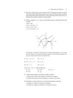
This has a nice graphical representation. (See Figure 22.11.) On each subinterval, the
difference between the rectangles from R
n
and L
n
is a small “difference” rectangle. Sliding
all these difference rectangles over to one side forms a total difference rectangle with height
v(4) − v(1) = 13 − 7 = 6 and width t =
3
n
.Ast goes to zero, the area of this rectangle
representing the difference between the R
n
and L
n
must also go to zero.
720 CHAPTER 22 Net Change in Amount and Area: Introducing the Definite Integral
v(t)
t
v(t)
t
1
4

123
4
13
7
6
(4, 13)
(1, 6)
∆t
Difference rectangles
Figure 22.11
The rectangles for the upper bound lie above the velocity curve and the rectangles for
the lower bound lie below the velocity curve. If the difference between the two bounds
approaches zero, the area of each set of rectangles must be approaching the area under the
velocity curve.
To summarize, because v(t) is increasing, R
n
(the right-hand sum) will always give an
upper bound for the cheetah’s net change in position and L
n
(the left-hand sum) will always
give a lower bound.
L
n
< net change in position <R
n
Similarly, because v(t) is increasing
L
n
< the area under v(t) on [1, 4] <R
n

.
But lim
n→∞
(R
n
− L
n
) = 0, so lim
n→∞
R
n
= lim
n→∞
L
n
= the area under v(t) on [1, 4]
by the Squeeze Theorem.
This means that our conjecture is true. To compute the net change exactly, we need to find
the area under the curve v(t) between t = 1 and t = 4. In this particular example this region
is a trapezoid so we can compute its area easily.
area =
1
2
(height
1
+ height
2
) · (base)
=
1

2
(7 + 13) · (3)
= 30 meters
v(t)
t
1
4
13
7
3
Figure 22.12
The cheetah’s net change in position over the time interval [1, 4] is 30 meters.
REMARK: In this example the function v(t) is linear and therefore the exact area under v(t)
was midway between Ln and Rn. Draw a picture to convince yourself that for a nonlinear
function this is generally not true.