Calculus: An Integrated Approach to Functions and their Rates of Change, Preliminary Edition Part 84 pdf

26.1 Approximating Sums: L
n
, R
n
, T
n
, and M
n
811
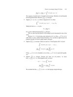
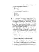
f
x
12345
f
x
12345
f
x
12
2
34 5
1 1.5 2 2.5 3 3.5 4 4.5 5
f
x
12345
f
x
12345
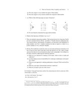
OR
midpoint rectangles midpoint tangent trapezoids
M
8

=
4
5
+
4
7
•
1
2
+
4
9
+
4
11
+
4
13
4
15
4
17
4
19
+ + +
(
(
= 1.599
L
8

=
1
1
+
2
3
•
1
2
+
2
4
+
2
5
+
2
6
2
7
2
8
2
9
+ + +
(
(
= 1.828
R
8

=
2
3
+
2
4
•
1
2
+
2
5
+
2
6
+
2
7
2
8
2
9
2
10
+ + +
(
(
= 1.428
T
8

=
L
8
+ R
8
= 1.628
We know that
1.428 =R
8
<M
8
=1.599 <

5
1
1
x
dx < T
8
= 1.628 <L
8
=1.828
f(x)=
1
x
is decreasing and concave up on [1, 5]. Therefore, we know that for any n
R
n
<


5
1
1
x
dx < L
n
and M
n
<

5
1
1
x
dx < T
n
.
If we are interested in more decimal places, we can simply choose larger values of n.
50 Subdivisions
Suppose n = 50; we chop [1, 5] into 50 equal pieces each of length x =
5−1
50
= 0.08. We
don’t actually want to sum up 50 terms by hand. Work like this is painful to do by hand
but it’s child’s play for a programmable calculator or computer. Get out your programmed
calculator or computer and check the figures given below.
5
R
50
= 1.577 M

50
= 1.60918 T
50
= 1.60994 L
50
= 1.641
400 Subdivisions
Suppose n = 400; we chop [1, 5] into 400 equal pieces each of length x =
5−1
400
= 0.01.
We obtain
R
400
= 1.60544 M
400
= 1.60943 T
400
= 1.60944 L
400
= 1.61344
Using T
400
as an upper bound and M
400
as a lower bound, we’ve nailed down the value
of this integral to 4 decimal places.
5
Yo u’ ll have to enter the following information: the function (often as Y
1

), the endpoints of integration, and the number of
pieces into which you’d like to partition the interval. (And, if you’re using a calculator without L
n
, R
n
, T
n
, and M
n
programmed,
you’ll have to enter the program.)
812 CHAPTER 26 Numerical Methods of Approximating Definite Integrals
REMARK M
50
and T
50
give better approximations of

5
1
1
x
dx than do R
400
and L
400
.
◆
Summary of the Underlying Principles
R

n
M
n
T
n
M
n
T
n
R
n
L
n
L
n
If f is increasing on [a, b], then L
n
<

b
a
f(t)dt <R
n
.
If f is decreasing on [a, b], then R
n
<

b
a

f(t)dt <L
n
.
If f is concave up on [a, b], then M
n
<

b
a
f(t)dt <T
n
.
If f is concave down on [a, b], then T
n
<

b
a
f(t)dt <M
n
.
For any given n, generally the trapezoidal and midpoint sums are much closer to the actual value of the
definite integral than are the left- and right-hand sums.
◆
EXAMPLE 26.2 Approximate

2
0
e
−2x

2
dx by finding upper and lower bounds differing by no more than
0.001.
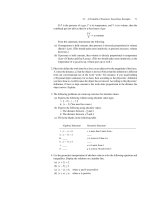
6
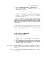
SOLUTION This is a great problem on which to practice, because it is impossible to find an antiderivative
for f(x)=e
−2x
2
unless we resort to an infinite sum of terms. Look at the graph of f(x).It
is decreasing on the interval [0, 2] and appears to have a point of inflection somewhere on
this interval.
7
f
x
1
12
f(x) = e
–2x
2
Figure 26.8
Suppose we were planning to use left- and right-hand sums only. As shown in Sec-
tion 22.2, the difference between the left- and right-hand sums is given by
6
The function e
−kx
2
is of practical importance because, for the appropriate k, its graph gives the bell-shaped normal distribution
curve. The area under the normal distribution curve over some given interval is of vital importance to probabilists and statisticians.
7
How can we be sure f is decreasing? f(x)=

1
e
2x
2
.Asxincreases from 0 to 2, 2x
2
increases, so e
2x
2
is positive and increasing.
Therefore, its reciprocal is decreasing. Alternatively,
d
dx
e
−2x
2
= e
−2x
2
(−4x) =
−4x
e
2x
2
≤ 0 for 0 ≤ x ≤ 2.
26.1 Approximating Sums: L
n
, R
n
, T

n
, and M
n
813
|R
n
− L
n
|=|f(b)−f(a)|·x
=|f(b)−f(a)|·
b−a
n
.
Therefore, in this example
|R
n
− L
n
|=|e
−8
−e
0
|·
2−0
n
=|e
−8
−1|·
2
n

<
1.9994
n
.
If we want |R
n
− L
n
| < 0.001, then we can solve
1.9994
n
= 0.001 for n and choose any integer
larger than this.
n =
1.9994
0.001
= 1999.4,
so we can choose n = 2000.
If your calculator will accept a number this large, you’re in good shape; the left-hand
sum will be an upper bound and the right-hand sum will be a lower bound, because f is de-
creasing on [0, 2]. The computation may take some time for the machine to perform, depend-
ing upon its power. You should get L
2000
= 0.62711719 and R
2000
= 0.62611753
REMARK Suppose f is monotonic
8
over the interval [a, b], so the actual value of


b
a
f(x)dx
is between L
n
and R
n
. Although it is possible simply to try larger and larger values of n
until L
n
and R
n
are within the desired distance from one another, it is more efficient, if a
high degree of accuracy is demanded, to use
|R
n
− L
n
|=|f(b)−f(a)|x
to find an appropriate value of n.
Generally, the midpoint and trapezoidal sums give us much better bounds for a partic-
ular n.Ifwefind the point of inflection, we can use these sums to form a sandwich around
the value of the integral.
f(x)=e
−2x
2
f

(x) =−4xe
−2x

2
f

(x) =−4[e
−2x
2
+ x(−4xe
−2x
2
)]
= 4e
−2x
2
(−1 + 4x
2
)
f

(x) = 0, where −1 + 4x
2
= 0, that is, where x
2
=
1
4
. On [0, 2] f

(x) = 0atx=
1
2

.
Looking back at f

(x) = 4e
−2x
2
(−1 + 4x
2
), we can see that f

changes sign (from
negative to positive) at x =
1
2
,sox=0.5 is a point of inflection. f is concave down on
[0,
1
2
] and concave up on [
1
2
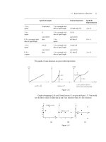
, 2]. Therefore,
8
f is monotonic on [a, b] if it is either always increasing on [a, b] or is always decreasing on [a, b].
814 CHAPTER 26 Numerical Methods of Approximating Definite Integrals
on [0,
1
2
], T
n

gives a lower bound for the integral and M
n
gives an upper bound;
on [
1
2
, 2], T
n
gives an upper bound for the integral and M
n
gives a lower bound.
f
x
1
1
2
21
f(x) = e
–2x
2
Figure 26.9
The combined error on [0,
1
2
] and [
1
2
, 2] must be no more than 0.001. We can split up the
allowable error however we want. We can play around with the calculator or computer until
the sum of |T

n
− M
n
| on [0,
1
2
] and |T
m
− M
m
| on [
1
2
, 2] is less than 0.001.
Here is the result of some playing around. If we try n = 50 on both intervals, we obtain
the following.
On [0,
1
2
] T
50
= 0.427802 M
50
= 0.4278170
On [
1
2
,2] T
50
= 0.198895 M

50
= 0.198759
On each interval the difference between T
50
and M
50
is substantially less than 0.0005. To
get the final answer we need to add the lower bounds (T
50
on [0,
1
2
] and M
50
on [
1
2
, 2]) to
obtain a lower bound for the integral, and add the upper bounds to obtain an upper bound.

2
0
e
−2x
2
dx =

.5
0
e

−2x
2
dx +

2
.5
e
−2x
2
dx
lower bound: 0.427802 + 0.198759 = 0.627065
upper bound: 0.428170 + 0.198895 = 0.627065
In the next section we will show an alternative and more efficient method of using the
trapezoidal and midpoint sums to approximate this integral.
◆
Numerical methods of integration, such as left- and right-hand sums and trapezoidal
and midpoint sums, are very useful not only when we are trying to approximate

b
a
f(x)dx
and can’t find an antiderivative for f , but also in situations in which we don’tevenhavea
formula for f . A scientist may be taking periodic data readings, or a surveyor may be taking
measurements at preset intervals, and these data sets may constitute the only information
we have about f . Numerical methods of integration can be applied directly to the data sets.
Exercise 26.1 below deals with information from a data set, and the results of Exercise 26.2
and Exercise 26.3 can be easily applied to data sets in which data have been collected at
equally spaced intervals.
EXERCISE 26.1 Between noon and 5:00 p.m. water has been leaving a reservoir at an increasing rate. We
do not have a rate function at our disposal, but we do have some measurements indicating

the rate that water has been leaving at various times. The information is given below. These
measurements were not taken at equally spaced time intervals.
26.1 Approximating Sums: L
n
, R
n
, T
n
, and M
n
815
Time noon 1:00 1:30 2:00 3:00 3:45 4:15 5:00
Rate out (in gal/hr) 140 160 170 200 250 270 280 300
(a) Find good upper and lower bounds on the amount of water that has left the reservoir
between noon and 5:00 p.m.
(b) Use a trapezoidal sum to approximate the amount of water that has left the reservoir
between noon and 5:00 p.m.
Answers are provided at the end of the section.
EXERCISE 26.2 Our aim is to approximate

b
a
f(x)dx when we do not have a formula for f(x).Our data
consist of a collection of measurements of f(x) taken at equally spaced intervals. Use a
trapezoidal sum to approximate the definite integral.
Partition the interval [a, b] into n equal subintervals, each of length x =
b−a
n
.
x

0
, x
1
, x
2
, ,are as indicated. x
0
= a and x
k
= a + kx for k = 1, ,n.y
k
=f(x
k
)for
k = 0, ,n.
Show that
the trapezoidal sum can be computed as follows:
T
n
=

1
2

[y
0
+ 2y
1
+ 2y
3

+···+2y
n−1
+y
n
]x.
x
1
x
0
y
0
y
1
a
x
2
x
3
x
4
x
n
x
n–1
y
n–1
y
n
b
=

=
Figure 26.10
The answer is provided at the end of the section.
Answers to Selected Exercises
Exercise 1
(a) The rate is increasing, so the lower bound is given by the left-hand sum and the upper
bound by the right-hand sum.
Lower bound: 140(1) + 160(0.5) + 170(0.5) + 200(1) + 250(0.75) + 270(0.5) +
280(0.25) = 897.5
Upper bound: 160(1) + 170(0.5) + 200(0.5) + 250(1) + 270(0.75) + 280(0.5) +
300(0.25) = 1012.5
Between 897.5 and 1012.5 gallons of water have left the reservoir.
816 CHAPTER 26 Numerical Methods of Approximating Definite Integrals
(b) The trapezoidal approximation is the average of the left- and right-hand sums given
above. The different lengths of the intervals do not change this basic principle. (Con-
vince yourself of this.)
Trapezoidal sum =
1
2
(897.5 + 1012.5) = 955
Exercise 2.
T
n
=
1
2
[(y
0
+ y
1

+ y
2
+ +y
n−1
)x + (y
1
+ y
2
+ y
3
+ +y
n
)x]
=
1
2
(y
0
+ 2y
1
+ 2y
2
+ +2y
n−1
+y
n
)x
PROBLEMS FOR SECTION 26.1
Some of the problems in this problem set require the use of a programmable calculator
or a computer. These are not highlighted in any way, but common sense should tell

you that summing a couple of hundred terms is not a good use of your time. On
the other hand, in order to make sure that you understand the numerical methods,
some problems explicitly ask you to refrain from using a program to execute the
computation.
1. Suppose we use right- and left-hand sums to approximate

b
a
f(t)dt.Wepartition the
interval [a, b] into n equal pieces each of length t. Let R
n
be the right-hand sum using
n subdivisions and L
n
be the left-hand sum using n subdivisions.
(a) Show that R
n
= L
n
+ f (b)t − f (a)t.
(b) Conclude that R
n
− L
n
= [f(b)−f(a)]t = [f(b)−f(a)]
|b−a|
n
.
2. (a) Find


x
1
1
t
dt, where x>0.
(b) ln x can be defined to be

x
1
1
t
dt. Sketch the graph of 1/t and approximate ln 2
numerically by partitioning the interval [1, 2] into 4 equal pieces and computing
L
4
and R
4
. Write out the sum long-hand, without using a calculator program.
(c) Into how many equal pieces would you have to subdivide the interval [1, 2] in order
to approximate ln 2 so that R
n
and L
n
give upper and lower bounds that differ by
no more than 0.01? Call this number p.
(d) Compute M
p
and T
p
.

(e) Into how many equal pieces would you have to subdivide the interval [1, 3] in order
to approximate ln 3 so that R
n
and L
n
give upper and lower bounds that differ by
no more than 0.001? That differ by no more than D?
3. Compute

e
1
ln xdxwith error less than 0.002. Try, by experimentation, to see how
many subdivisions are required for M
n
and T
n
to differ by less than 0.002. How many
are required for L
n
and R
n
to differ by less than 0.002?
26.1 Approximating Sums: L
n
, R
n
, T
n
, and M
n

817
4. (a) Let f be the function graphed below. f is increasing and concave down.
f
x
a
b
Let A =

b
a
f(x)dx. Suppose that estimates of f(x)dx are computed using the
left, right, and trapezoid rules, each with the same number of subintervals. We’ll
denote these estimates by L
n
, R
n
, and T
n
, respectively. Put the numbers A, L
n
,
R
n
, and T
n
in ascending order. Justify your answer and explain why your answer
is independent of the value of n used.
(b) Answer the same question as above if the graph of f is the one given below. f is
decreasing and concave up on [a, b].
f

x
a
b
5. Consider

4
1
√
xdx.
(a) Find a value of n for which



L
n
−

b
a
f(x)dx



≤0.01.
(b) Use the value of n from part (a) to find L
n
and R
n
.
(c) Is the average of the left- and right-hand sums larger than the integral, or smaller?

(d) Compare your numerical approximations to the answer you get using the Funda-
mental Theorem of Calculus.
6. Approximate

1
0
√
1 + x
4
dx with error less than 0.01.
7. Give upper and lower bounds for

2
0
10
2+x
5
dx such that the upper and lower bounds
differ by less than 0.01.
8. Give upper and lower bounds for

3
2
1
ln x
dx such that the two bounds differ from one
another by less than 0.05. Explain how you know that the upper bound is indeed an
upper bound and the lower bound is indeed a lower bound.
9. Consider


9
4
1
√
x
dx.
(a) Find a value of n for which
|
L
n
− R
n
|
≤ 0.01.
(b) Use that value of n to find L
n
and R
n
.
818 CHAPTER 26 Numerical Methods of Approximating Definite Integrals
(c) If you take the average of the left- and right-hand sums, will your approximation
be larger than the integral, or smaller?
(d) Compare your numerical approximations to the answers you get using the Funda-
mental Theorem of Calculus.
10. One of your friends is doing his mathematics homework on the run. He managed to
squeeze in one problem between lunch and his expository writing class. He used his
calculator to find L
n
, R
n

, T
n
, and M
n
to approximate a definite integral and jotted down
the results on a napkin. They were
0.367617, 0.3211885, 0.341189, and 0.274760.
He didn’t write down the problem, nor did he record the value of n he used. But he did
sketch the function (over the relevant interval) on the napkin; it looked like this.
f
x
He wants your help in labeling the data he recorded as a left-hand sum, a right-hand
sum, a midpoint sum, and a trapezoidal sum. Which is which? Explain your answer.
11. Measurements of the width of a pond are taken every 20 yards along its length. The
measurements are: 0 yards, 60 yards, 50 yards, 70 yards, 50 yards, and 30 yards.
Approximate the surface area of the pond using the Trapezoidal rule.
60
50
70
50
30
20
20 20 20 20
12. Approximate each of the following integrals with error less than 1/100.
(Note: If you look at all the questions and think about a strategy in advance, you
will only have to compute two integrals in order to answer all four questions with
the desired degree of accuracy. There is no problem with being more accurate than is
requested.) Briefly explain what you have done and how many subdivisions you used.
(i)


1
0
e
−(
1
2
)x
2
dx (ii)

2
1
e
−(
1
2
)x
2
dx (iii)

2
0
e
−(
1
2
)x
2
dx (iv)


2
−2
e
−(
1
2
)x
2
dx
26.1 Approximating Sums: L
n
, R
n
, T
n
, and M
n
819
13. Let f(x)=
3
x
3
+x
. Let a and b be positive constants, 0 <a<b.Below are two partitions
of the interval [a, b]. One (given with w’s) partitions [a, b] into 8 equal subintervals,
each of length w; the other (given with t’s) partitions the interval into 12 equal pieces
each of length t.
w
i
= a + iw, i = 0, 1, ,8

t
i
=a+it, i = 0, 1, ,12
Put the following expressions in ascending order, with “<” or “=” signs between them.
(Identify the sum with the letter preceding it.)
A =
7

i=0
f(w
i
)w B =
8

i=1
f(w
i
)w
C =
11

i=0
f(t
i
)t D =
12

i=1
f(t
i

)t
E =

b
a
f(w)dw F =f(a)·(b − a)
14. Approximate

2
−1
arctan xdxusing left- and right-hand sums to obtain an upper and
lower bound for the integral with difference less than 0.05. Save time by graphing
y = arctan x and using symmetry to simplify the problem.
15. The function f(x)is decreasing and concave down on the interval [3, 5]. Suppose that
you use a right-hand sum, R
100
, a left-hand sum, L
100
, a trapezoidal sum, T
100
, and a
midpoint sum, M
100
, all with 100 subdivisions, to estimate

5
3
f(x)dx. Select all of
the following that must be true.
(a) L

100
≥ R
100
(b)

5
3
f(x)dx ≥T
100
(c) T
100
≥ R
100
(d) T
100
≥ M
100
(e) M
100
≥ L
100
(f) T
100
= (L
100
+ R
100
)/2
16. Suppose that g is a differentiable function whose derivative is g


(x) =
2
x
2
+3
. Partition
[0, 2] into n equal pieces each of length x and let x
k
= kx, where k = 0, 1, ,n.Put
the following expressions in ascending order (with “<” or “=” signs between them).
A =
n

i=1
g(x
i
)x B =
n−1

i=0
g(x
i
)x
C = lim
n→∞
n−1

i=0
g(x
i

)x D = lim
n→∞
n

i=1
g(x
i
)x
820 CHAPTER 26 Numerical Methods of Approximating Definite Integrals
17. Suppose L
10
<

b
a
f(x)dx <R
10
and |R
10
− L
10
| < 0.01. Which of the following
statements must be true? Circle all such statements.
(a) |R
10
−

b
a
f(x)dx|<0.01 (b) |T

10
−

b
a
f(x)dx|<0.01
(c) |T
10
−

b
a
f(x)dx|<0.005 (d) |L
10
−

b
a
f(x)dx|<0.005
18. Two of the following three integrals you can evaluate exactly. One you cannot, until
learning integration by parts. Identify the one you cannot evaluate exactly and approx-
imate it with an error under 0.05. Find exact answers for the other two integrals.
(a)

e
1
ln x
x
dx (b)


1
0
xe
x
2
dx (c)

1
0
xe
x
dx
26.2 SIMPSON’S RULE AND ERROR ESTIMATES
Simpson’s Rule
We began our discussion with left- and right-hand sums, sums that provide bounds for

b
a
f(x)dx if f is monotonic on [a, b]. Then we came up with the clever idea of using
the average of L
n
and R
n
to approximate a definite integral. This led us to the trapezoidal
sum, which generally gives a much better approximation to a definite integral than either
the left or right sums for the same number of subdivisions. Encouraged by our success,
we might start thinking about averaging the midpoint and trapezoidal sums. An even
better idea would be to take a weighted average of these two sums. This is because the
midpoint rule generally gives us a better fit than does the trapezoidal rule. In fact, analysis
of numerical data indicates that the error in using the trapezoidal rule is about two times

the size as that from using the midpoint rule. From the picture below this seems plausible.
The weighting
M
n
+M
n
+T
n
3
=
2M
n
+T
n
3
gives us a method of approximating definite integrals
known as Simpson’s rule.
x
i
x
i +1
midpoint
=
=
Error using trapezoid
=
Error using midpoint
tangent trapezoid
The shaded area is about
double the blackened area.

Weighted average: weight
midpoint twice as
heavily as the
trapezoidal sum.
2M
n
+ T
n
3
Simpson's rule
Figure 26.11
Simpson’s rule: S
2n
=
2M
n
+ T
n
3