Calculus: An Integrated Approach to Functions and their Rates of Change, Preliminary Edition Part 85 potx

26.2 Simpson’s Rule and Error Estimates 821
We call it S
2n
because we need n data points for M
n
and (n + 1) different data points for
T
n
. Sometimes it will be convenient to write S
p
=
2M
n
+T
n
3
where p = 2n.
Simpson’s rule generally gives a substantially better numerical estimate than either
the midpoint or the trapezoidal sums. To get some appreciation for this, try it out on some
integrals that you can compute exactly. Below we do this for the integral

5
1
1/x dx.
◆
EXAMPLE 26.3 Compare M
n
, T
n
, and Simpson’s rule (the weighted average) for


5
1
1
x
dx, where n = 4, 8,
50, and 100. Note that

5
1
1
x
dx = ln |x|



5
1
= ln 5 − ln 1 = ln 5 = 1.60943791
SOLUTION (a) n = 4: M
4
= 1.57460
T
4
=1.68333
Simpson’s rule =
2M
4
+T
4
3

= 1.61084
(b) n = 8: M
8
= 1.59984
T
8
=1.62896
Simpson’s rule =
2M
8
+T
8
3
= 1.60955
(c) n = 50: M
50
= 1.60918221
T
50
= 1.60994957
Simpson’s rule =
2M
50
+T
50
3
= 1.60943799
(d) n = 100: M
100
= 1.60937393

T
100
= 1.60956589
Simpson’s rule =
2M
100
+T
100
3
= 1.60943791
◆
Like the trapezoidal sum, Simpson’s rule is a convenient tool for approximating

b
a
f(x)dx even when a formula for f is not available. For instance, the values of f(x)
referred to in the discussion below could be measurements taken by a surveyor estimating
the area of a plot of land or body of water.
Suppose our aim is to approximate

b
a
f(x)dx.Wecan collect values of f(x)at equally
spaced intervals and use Simpson’s rule to approximate the definite integral. Partition the
interval [a, b] into n equal subintervals, each of length x =
b−a
n
. We need to use a weighted
average of the midpoint and trapezoidal sums; therefore, on each subinterval we need not
only the value of f at each endpoint (for T

n
) but also the value of f in the middle (for M
n
).
Although we are chopping [a, b] into n equal subintervals, we will use 2n + 1 values of f
(n + 1 values for T
n
and n values for M
n
).
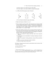
Let y
k
= f(x
k
)for k = 0, ,2n,where x
0
, x
1
, x
2
, ,x
2n
are as indicated below.
x
k
= a + k

x
2


for k = 0.1, ,2n
x
0
a
x
1
x
2
x
3
x
4
x
2n–2
x
2n–1
x
2n
∆ x ∆ x ∆ x
=
b
=
for M
n
for M
n
. . .
for M
n
Figure 26.12

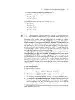
In the following exercise you will show that using this labeling convention, Simpson’s
rule can be used to approximate the definite integral using the following formula.
822 CHAPTER 26 Numerical Methods of Approximating Definite Integrals
Simpson’s rule:
S
2n
=

1
6

[y
0
+ 4y
1
+ 2y
2
+ 4y
3
+ 2y
4
+···+2y
2n−2
+4y
2n−1
+y
2n
]x,
where x =
b − a

n
.
EXERCISE 26.3 In this exercise use the labeling system described above: Partition [a, b] into n equal pieces
of length x =
b−a
n
.
x
k
= a + k

x
2

for k = 0, 1, ,2n, where x =
b − a
n
Let y
k
= f(x
k
)for k = 0, ,2n,where x
0
, x
1
, x
2
, ,x
2n
.

(a) Show that using this labeling convention
T
n
=

1
2

(y
0
+ 2y
2
+ 2y
4
+ 2y
6
+···+2y
2n−2
+y
2n
)x.
(b) Show that using this labeling convention
M
n
= (y
1
+ y
3
+ y
5

+ y
7
+···+y
2n−1
)x.
(c) Show that using this labeling convention Simpson’s rule is given by

1
6

(y
0
+ 4y
1
+ 2y
2
+ 4y
3
+ 2y
4
+···+2y
2n−2
+4y
2n−1
+y
2n
)x.
The answer to part (c) is given at the end of the section.
Notice that because Simpson’s rule requires both the midpoint and trapezoidal rules and
the relevant data points for each of these two rules are different, Simpson’s rule requires

approximately double the number of data points necessary for computing either M
n
or T
n
individually.
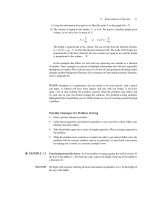
REMARKS
Simpson’s rule can be presented without reference to the trapezoidal and the midpoint
sums. Instead, it can be viewed as follows. On each subinterval [x
i−1
, x
i
] approximate
the area under f by the area under the parabola passing through the three points on
the graph of f corresponding to the endpoints of the interval and the midpoint, or
(x
i−1
, f(x
i−1
)), (x
i
, f(x
i
)), and

x
i−1
+x
i
2
, f


x
i−1
+x
i
2

.
26.2 Simpson’s Rule and Error Estimates 823
x
i–1
x
i+1
x
i
A
B
C
D
E
Find a parabola through A, B, and C.
Find another parabola through
C, D, and E.
Sum the areas under the parabolas to
approximate the area under the curve.
Figure 26.13
When Simpson’s rule is applied to cubics, it will always give an exact answer, even
when using
2M
1

+T
1
3
.
Error Bounds
In Section 26.1 we used approximating sums to provide upper and lower bounds for the
value of an integral. When we use Simpson’s rule we have a “good” estimate, but without
getting a bound on the error involved we cannot be sure how “good” the estimate is. While
we cannot expect to know the exact error in using approximating sums, it would be quite
useful to get a bound on the error. Consider, for instance, Example 26.2. It would be useful
to be able to approximate

2
0
e
−2x
2
dx using the trapezoidal rule or Simpson’s rule, having
a bound for the error but not worrying about the point of inflection.
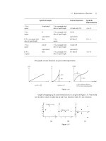
Let’s begin by thinking about the error involved in using left- and right-hand sums.
y
x
13
y
x
13
y
x
13
The steeper the slope of f the larger the error in approximating by rectangles.

Figure 26.14
As illustrated in Figure 26.14, the larger |f

| is, the larger the magnitude of the error involved
in approximating the area under the curve by the area of a rectangle.
When approximating the area using the trapezoidal rule or the midpoint tangent trape-
zoid, the magnitude of f

is not an issue; the rate that f

is changing, (measured by f

), is
a factor controlling the error.
For L
n
, R
n
, T
n
, and M
n
, the larger n is, the smaller the expected error. Put another
way, the smaller x is, the smaller the expected error. Using the Mean Value Theorem, the
following error bounds can be proven.
824 CHAPTER 26 Numerical Methods of Approximating Definite Integrals
Let I =

b
a

f(x)dx.Let L
n
, R
n
, T
n
, and M
n
be left, right, trapezoidal, and midpoint
approximations of I , respectively. Then
|L
n
− I |≤
M
1
(b − a)
2
2n
where M
1
is the maximum value of |f

| on [a, b].
|R
n
− I |≤
M
1
(b − a)
2

2n
|T
n
− I |≤
M
2
(b − a)
3
12n
2
where M
2
is the maximum value of |f

| on [a, b].
|M
n
− I |≤
M
2
(b − a)
3
24n
2
You might guess that the error bound for Simpson’s rule involves an n
3
and the third
derivative of f . In fact, Simpson’s rule is much more accurate than you might expect. It
can be shown that
|S

2n
− I |≤
M
4
(b − a)
5
180(2n)
4
where M
4
is the maximum value of |f
(4)
| on [a, b].
If p is an even number, then
|S
p
− I |≤
M
4
(b − a)
5
180p
4
.
◆
EXAMPLE 26.4 Find upper bounds for the error involved in using T
10
and M
10
to approximate


2
0
e
−2x
2
dx.
SOLUTION In order to use the error estimates for T
10
and M
10
we need to find an upper bound for f

on [0, 2]. In Example 26.2 we computed f

(x).Iff(x)=e
−2x
2
,then
f

(x) = 4e
−2x
2
(−1 + 4x
2
)
=
4(−1 + 4x
2

)
e
2x
2
.
We can get a crude upper bound for f

on [0, 2] by noting that the numerator is no more
than 4(−1 + 4 · 2
2
) = 4(−1 + 16) = 15 · 4 = 60.
|f

(x)|≤
60
e
2x
2
= 60e
−2x
2
e
−2x
2
≤ 1on[−0, 2] so
|f

(x)| < 60.
NOTE We haven’t found M
2

, but we found a bound for M
2
.
|T
10
− I |≤
M
2
(b − a)
3
12n
2
where a = 0, b = 2, n = 10, and M
2
< 60
|T
10
− I | <
60 · 2
3
12 · 100
=
480
1200
= 0.4
The error using T
10
is guaranteed
to be less than 0.4.
|M

10
− I | <
60 · 2
3
24 · 100
=
0.4
2
= 0.2
The error using M
10
is guaranteed
to be less than 0.2.
◆
26.2 Simpson’s Rule and Error Estimates 825
◆
EXAMPLE 26.5 How big should n be to easily guarantee that M
n
approximates

2
0
e
−2x
2
dx to within 0.001?
SOLUTION From Example 26.4 we know that |M
n
− I| <
480

24n
2
=
20
n
2
. We must find n such that
20
n
2
< 0.001. We’ll solve
20
n
2
= 0.001 and pick the next higher integer.
n
2
(0.001) = 20 =>n
2
=20,000 Then n ≈ 141.4.
So we choose n = 142.
◆
◆
EXAMPLE 26.6 Get an upper bound for the error involved in using S
10
to approximate ln 3 =

3
1
1

x
dx.
SOLUTION f(x)=
1
x
. Compute f

, f

, f

, and f
(4)
. Confirm that f
(4)
(x) =
24
x
5
.
On [1, 3],




24
x
5





≤ 24.
|S
p
− I |≤
M
4
(b − a)
5
180p
4
where a = 1, b = 3, p = 10, and M
4
= 24.
≤
24(3 − 1)
5
180 · 10
4
≤
24 · 2
5
18 · 10
5
< 4.27 × 10
−4
≈ 0.00043
◆
Answers to Selected Exercises

Exercise 26.3(c)
Simpson’s rule =
2M
n
+T
n
3
=

1
3

[2(y
1
+ y
3
+ y
5
+···+y
2n−1
)x +

1
2

(y
0
+ 2y
2
+ 2y

4
+ 2y
6
+···+2y
2n−2
+y
2n
)x]
= [2y
1
+ 2y
3
+ 2y
5
++···+2y
2n−1
)]·x ·

1
3

+
[y
0
+ 2y
2
+ 2y
4
+ 2y
6

+···+2y
2n−2
+y
2n
)]

1
2

x ·

1
3

= [4y
1
+ 4y
3
+ 4y
5
+···+4y
2n−1
)]·

1
6

x + [y
0
+ 2y

2
+ 2y
4
+ 2y
6
+···+2y
2n−2
+y
2n
)]·

1
6

· x
= [y
0
+ 4y
1
+ 2y
2
+ 4y
3
+ 2y
4
+ 4y
5
+ 2y
6
+ 4y

7
+···+2y
2n−2
+4y
2n−1
+y
2n
)]·

1
6

x
826 CHAPTER 26 Numerical Methods of Approximating Definite Integrals
PROBLEMS FOR SECTION 26.2
1. Approximate

e
1
ln xdx using Simpson’s rule with p = 10. S
10
=
2M
5
+T
5
3
. Find an
upper bound for the error. At a certain point you’ll use the fact that e<3.
2. Approximate the following integrals using the trapezoidal rule, the midpoint rule, and

Simpson’s rule for the specified number of subdivisions and compute error bounds
using the formulas given in this section. Compare your answers to the exact answer.
(a)

2
0
x
2
dx n = 4 (b)

1
0
1
x+1
dx n = 4
3. Approximate the following integral using the trapezoidal rule, the midpoint rule, and
Simpson’s rule for the specified number of subdivisions. Look at T
n
, M
n
, and S
2n
.
Compute error bounds.

2
1
ln xdx (a) n = 4 (b) n = 8 (c) n = 10
4. (a) Approximate


1
0
cos(x
2
)dxusing M
10
. Find an upper bound for the error.
(b) Approximate

1
0
cos(x
2
)dx using S
20
. S
20
=
2M
10
+T
10
3
. Find an upper bound for
the error.
5. A surveyor is measuring the cross-sectional area of a 30-foot-wide river beneath a
bridge. He measures the river’s depth every 5 feet. The data are given below.
Depth (in feet) 0.5
5 ft


1.5
5 ft

3
5 ft

5
5 ft

4
5 ft

3
5 ft

1
(a) Use the trapezoidal sum to approximate the cross-sectional area of the river.
(b) Use Simpson’s rule to approximate the cross-sectional area of the river.
27
CHAPTER
Applying the Definite Integral:
Slice and Conquer
27.1 FINDING “MASS” WHEN DENSITY VARIES
Up to this point we’ve used the definite integral to
find the signed area under the graph of f and
find the net change in amount when given a rate function.
In this chapter we will see how the idea of slicing that led us to the limit definition
of the definite integral can help us apply our knowledge about definite integrals to other
situations.
◆

EXAMPLE 27.1 A geologist is working with a rectangular block-shaped chunk of sedimentary rock whose
height is 3 meters, width is 4 meters, and length is 7 meters. A certain mineral is uniformly
distributed throughout the rock sample with a density of 5 milligrams per cubic meter. How
many milligrams of the mineral are in the sample?
SOLUTION To calculate the number of milligrams given the density we simply multiply volume by
density. The volume of the rock is length · width · height = (7 m) · (4 m) · (3 m) = 84 m
3
.
Therefore,
number of grams of the mineral = 84 m
3
· 5
mg
m
3
= 420 mg.
Notice that the units of volume cancel to leave an answer in milligrams.
◆
◆
EXAMPLE 27.2 The geologist is now looking at another mineral in the same sedimentary rock sample. This
mineral had begun to settle as the rock was being formed, so its density varies with depth.
The density is given by ρ(h) = 1 + 0.1h
2
milligrams per cubic meter, where h is the depth
827
828 CHAPTER 27 Applying the Definite Integral: Slice and Conquer
below the top surface of the sample.
1
Notice that as the depth h increases, so does the density
of the mineral in the rock sample. We want to find the number of milligrams of this mineral

in the sample.
SOLUTION Compare this problem to the first one. The difficulty is that the density is not constant; it
varies from ρ(0) = 1 mg/m
3
at the top of the sample to ρ(3) = 1.9 mg/m
3
at the bottom. If
we were to multiply the total volume of the rock sample by ρ(0), we would get 84 mg; if we
were to multiply the total volume of the rock sample by ρ(3), we would get 159.6 mg. The
former number is much too small and the latter is much too big. The actual number of grams
of the mineral must be somewhere between these two extremes. How can we improve upon
our under- and overestimates?
At any fixed depth the density is constant. Suppose we divide the sample into horizontal
slabs, slices in which the density doesn’t vary much. In each slice we can approximate the
number of milligrams of the mineral; we’ll add up the estimates in each slice to approximate
the total number of milligrams. The finer the slices, the less the density will vary within a
slice and the better our approximation will be.
Notice that this strategy is the same one we successfully applied to the problem of
finding the area under a curve. In the area problem our dilemma was that the function f
varied with x over the x-interval [a, b]. To deal with this we chopped the interval [a, b]
into n equal pieces, on each piece approximated the function by a constant, used that to
approximate the area on the subinterval, and summed these areas. We found the area under
the curve by letting the number of subintervals grow without bound. Here our dilemma
is that the density varies with h,sowe’ll partition the h-interval [0, 3] into pieces, thereby
partitioning the rock sample into thin horizontal slabs in which density doesn’t vary greatly.
Approximating the Number of Milligrams of Mineral in the Sample
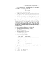
Suppose we divide the h-interval [0, 3] into six equal subintervals. Using the notation we
developed for Riemann sums, these are [h
0
, h

1
] through [h
5
, h
6
], where the height of each
subinterval is h = 0.5 m and h
i
= ih for i = 0, 1, ,6. This chops the entire rock
sample into six slabs, each of which has height 1/2 meter, width 4 meters, and length 7
meters, as shown in Figure 27.1.
h
0
= 0
h
1
= .5
h
2
= 1
h
3
= 1.5
h
4
= 2
h
5
= 2.5
h

6
= 3
h
0
= 0
h
1
= .5
h
2
= 1
h
3
= 1.5
h
4
= 2
h
5
= 2.5
h
6
= 3
7 m
3 m
4 m
∆h = 0.5 m {
Figure 27.1
We can estimate the number of milligrams of mineral in each slice. For example, in the
top slice, the density varies from ρ(0) = 1 + 0.1(0)

2
= 1 mg/m
3
at the top surface to
ρ(0.5) = 1 + 0.1(0.5)
2
= 1.025 mg/m
3
at the bottom surface. The volume of the slice is
1
The Greek letter ρ, pronounced “rho,” is often used in the sciences to represent density.
27.1 Finding “Mass” When Density Varies 829
(4 m)(7 m)(h m) = (4)(7)(0.5) m
3
= 14 m
3
. The density increases with h,sowehavethe
following estimates for the number of milligrams of mineral in this top slice.
underestimate: ρ(0) · (volume of slice) = 1
mg
m
3
· 14 m
3
= 14 mg
overestimate: ρ(0.5) · (volume of slice) = 1.025
mg
m
3
· 14 m

3
= 14.35 mg
We follow the same procedure for each of the five other slices. Then, by adding all
the underestimates for the separate slices, we obtain an underestimate for the total number
of milligrams in the sample. Similarly, adding the overestimates on all six slices gives an
overestimate for the total.
underestimate =
5

i=0
ρ(h
i
) · [28 · h]
=
5

i=0
(1 + 0.1h
2
i
) · [28 · h]
= 103.25 mg
overestimate =
6

i=1
ρ(h
i
) · [28 · h]
=

6

i=1
(1 + 0.1h
2
1
) · [28 · h]
= 115.85 mg
Notice that our method of slicing horizontally along the axis of the independent variable
h ensured that the density would not vary as much within each slice as it had in the rock
sample as a whole; this is what brought our estimates closer together. To slice vertically
would have defeated the purpose of slicing, because the density in each slice would still
have varied between ρ(0) and ρ(3), the same variance as in the entire rock sample.
KEY NOTION The choice of how to slice is at the heart of this kind of problem. This choice
is determined by the density function. In this case, the density varies with height, so we
need to slice in a way that keeps the height (and hence the density) approximately constant
within each slice.
Computing the Exact Number of Milligrams in the Sample
We can improve upon our estimates by partitioning the h-interval [0, 3] into finer and finer
subintervals; this corresponds to cutting thinner and thinner horizontal slabs of the rock
sample. As we let the number of subintervals grow without bound, we expect the difference
between the overestimates and the underestimates to tend toward zero, just as it did in the
area problem.
Chop the h-interval [0, 3] into n equal subintervals each of height h =
3
n
m and label
h
0
, h

1
, h
2
, ,h
n
as shown. h
i
= (i)
3
n
for i = 0, 1, ,n.This corresponds to slicing the
rock sample horizontally into n slabs, each 7 meters long by 4 meters wide by h meters
tall; the volume of each slice is (area) · (thickness) = 28h m
3
.
830 CHAPTER 27 Applying the Definite Integral: Slice and Conquer
∆h
h
a
–
h
i
–
h
n
–
4
7
Figure 27.2
Let’s look at a generic slice, say the ith slice.


the#ofmg
in the ith slice

≈

estimate of density of
the mineral in the slice

· (volume of the slice)
≈ ρ(h
i
)
mg
m
3
· (28h m
3
) (using ρ(h
i
) gives an overestimate)
≈ ρ(h
i
) · 28h mg
Thus, we obtain the following sums to estimate the total number of milligrams of the mineral
in the sample.
underestimate =
n−1

i=0

ρ(h
i
) · [28 · h] =
n−1

i=0
28ρ(h
i
) · h
overestimate =
n

i=1
ρ(h
i
) · [28 · h] =
n

i=1
28ρ(h
i
) · h
These sums are Riemann sums. The difference between the overestimate and the un-
derestimate is 28[ρ(h
n
) − ρ(h
0
)] · h. This can be written as 28[ρ(3) − ρ(0)] · h or
28(0.9)


3
n

=
75.6
n
.Asngrows without bound this difference tends toward zero; the limit
of the Riemann sums is the definite integral

3
0
ρ(h) · 28 dh.
We now calculate.
number of milligrams in sample = lim
n→∞
n

i=1
ρ(h
i
) · [28 · h] (= lim
n→∞
n−1

i=0
ρ(h
i
) · [28 · h])
=


3
0
ρ(h) · 28 dh
(Both sums approach the
value of the integral.)
=

3
0
(1 + 0.1h
2
) · 28 dh
= 28

h + 0.1
h
3
3





3
0
= 28

(3 + 0.9) − (0)

= 109.2 mg

The strategy of slicing, approximating, summing, and then taking a limit of the sum
allowed us to arrive at an exact answer.
◆