Calculus: An Integrated Approach to Functions and their Rates of Change, Preliminary Edition Part 96 pptx

30.1 Approximating a Function by a Polynomial 931
Alternating signs:
(−1)
k
and (−1)
k+1
can be used to indicate alternating signs. Which is needed to do the
job is determined by the notational system you happen to have chosen. The simplest
way of determining which you need is by trial and error. Try (−1)
k
and check it with
a particular k-value. If it doesn’t work, switch to (−1)
k+1
.
◆
EXAMPLE 30.5 Approximate
5
√
34 using the appropriate second degree Taylor polynomial.
SOLUTION Let f(x)=x
1
5
. We must center the Taylor polynomial at a point near 34 at which the values
of f , f

, and f

can be readily computed.
An off-the-cuff approximation of
5
√

34 is
5
√
34 ≈
5
√
32 = 2; we know that
5
√
34 is a bit
more than 2. Center the Taylor polynomial at x = 32.
P
2
(x) = f(32) + f

(32)(x − 32) +
f

(32)
2!
(x − 32)
2
f(x)=x
1
5
f(32) = 2
f

(x) =
1

5
x
−
4
5
f

(32) =
1
5
1
32
4
5
=
1
5
1
2
4
=
1
80
f

(x) =
−4
25
x
−

9
5
f

(32) =
−4
25
1
2
9
=
−1
25 · 2
7
=
−1
3200
Therefore,
P
2
(x) = 2 +
1
80
(x − 32) −
1
6400
(x − 32)
2
.
5

√
34 ≈ P
2
(34) = 2 +
1
80
(2) −
4
6400
= 2 +
1
40
−
1
1600
= 2.024375
This agrees with the actual value of
5
√
34 to four decimal places. ◆
If you study closely the numerical data in this section you can start to get a sense of
the magnitude of the error involved in a Taylor polynomial approximation. The size of the
error can be estimated by graphing f(x)−P
n
(x) using a calculator or computer. In the next
section we will state Taylor’s Theorem, which will provide not only a method of estimating
errors independent of a calculator, but also an invaluable theoretical tool.
PROBLEMS FOR SECTION 30.1
For Problems 1 through 7, do the following.
(a) Compute the fourth degree Taylor polynomial for f(x)at x = 0.

(b) On the same set of axes, graph f(x),P
1
(x), P
2
(x), P
3
(x), and P
4
(x).
(c) Use P
1
(x), P
2
(x), P
3
(x), and P
4
(x) to approximate f(0.1) and f(0.3). Compare
these approximations to those given by a calculator.
1. f(x)=e
−x
2. f(x)=ln(1 + x)
3. f(x)=tan
−1
x
932 CHAPTER 30 Series
4. f(x)=(1+x)
4
5. f(x)=
√

1 + x
6. f(x)=2x
4
−3x
2
+x −1
7. f(x)=(1+x)
−2
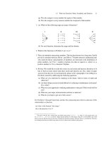
8. Below is a graph of f(x). For each quadratic given, explain why the quadratic could
not be the second degree Taylor polynomial for f(x)at x = 0.
(a) 2 + 3x −
1
2
x
2
(b) −1 − 5x + 2x
2
(c) −2 + 2x −
1
3
x
2
y
x
y = f(x)
9. Let P
2
(x) = a
0
+ a

1
x + a
2
x
2
be the second degree Taylor polynomial generated by
f(x)at x =0, where the graph of f is the one given in Problem 8 above. Use the graph
to determine the signs of a
0
, a
1
, and a
2
.
10. (a) Find the second degree Taylor polynomial generated by sec x at x = 0.
(b) Graph P
2
(x) and sec x on the same set of axes.
11. (a) Compute the third degree Taylor polynomial for tan x about x = 0.
(b) Why is it reasonable to expect the coefficient of the x
2
term to be zero?
12. The graph of a differentiable function f(x) is given. Use the graph to determine the
signs of the coefficients of the second degree Taylor polynomials indicated. f has a
minimum at x = 0 and a point of inflection at x = 2.
(a) P
2
(x) = a
0
+ a

1
x + a
2
x
2
(b) P
2
(x) = a
0
+ a
1
(x − 1) + a
2
(x − 1)
2
(c) P
2
(x) = a
0
+ a
1
(x − 2) + a
2
(x − 2)
2
(d) P
2
(x) = a
0
+ a

1
(x − 3) + a
2
(x − 3)
2
30.1 Approximating a Function by a Polynomial 933
y
x
y = f(x)
123
13. Let f(x)=ln(1 + x). Find the nth degree Taylor polynomial generated by f about
x = 0.
14. Compute the nth degree Taylor polynomial expansion of f(x)=
1
x
about x = 1. Graph
f and P
1
, P
2
, P
3
, and P
4
on a common set of axes.
In Problems 15 through 18, use a second degree Taylor polynomial centered appropri-
ately to approximate the expression given.
15.
3
√

8.3
16.
√
103
17. tan
−1
(0.75)
18.
3
√
29
19. Compute the third degree Taylor polynomial generated by sin x at x =
π
4
.
20. Find the fifth degree Taylor polynomial for
√
x centered at x = 9.
21. Write the third degree Taylor polynomial centered about x = 0 for f(x)=
1
(1+x)
p
,
where p is constant.
Introduction to Error Analysis: Problems 22 and 23.
22. Let f(x)=e
x
.Use the data given in the table on page 928 to compute the following.
(a) f(0.1) − P
k

(0.1) for k = 1, 2, ,5
(b) f(0.2) − P
k
(0.2) for k = 1, 2, ,5
(c) f(0.5) − P
k
(0.5) for k = 1, 2, ,5
(d) f(1)−P
k
(1) for k = 1, 2, ,5
Compare the size of the difference between the actual value of the function and the poly-
nomial approximation with that of the first “unused” term of the Taylor polynomial—
that is, the last term of the next higher degree polynomial—and observe that they have
the same order of magnitude.
934 CHAPTER 30 Series
23. Let f(x)=e
x
and let P
k
(x) be its kth degree Taylor polynomial about x = 0. Graph
R
k
(x) = f(x)−P
k
(x) for k =1, 2, ,5.
24. Use a third degree Taylor polynomial to approximate ln 0.9.
25. f(x)=12 + 3(x − 1) + 5(x − 1)
2
+ 7(x − 1)
3

. Find the following.
(a) f

(1) (b) f

(1) (c) f

(1) (d) f(1)
26. f(x)=
√
3 + 12(x − 5)
3
+ 17(x − 5)
6
. Find the following.
(a) f(5) (b) f

(5) (c) f

(5) (d) f
(6)
(5)
27. Compute the sixth degree Taylor polynomial generated by sin x about x = π.
28. Compute the sixth degree Taylor polynomial generated by cos x about x =−
π
2
.
29. Let f(x)=(1+x)
p
, where p is a constant, p = 0, 1, 2, 3, 4, 5.

(a) Compute the third degree Taylor polynomial for f(x)around x = 0.
(b) Compute the fifth degree Taylor polynomial for f(x)around x = 0.
30. Using the results of Problem 29(a), approximate the following. Compare your results
with the numerical approximations given by a calculator.
(a)
√
1.002 (b)
1
1.03
(c)
3
√
1.001
30.2 ERROR ANALYSIS AND TAYLOR’S THEOREM
An approximation is of limited use unless we have a notion of the magnitude of the error
involved. Every Taylor polynomial P
n
(x) has an associated error function, R
n
(x),defined
by
f(x)= P
n
(x) + R
n
(x)
function =

polynomial
approximation


+

associated
error

R
n
(x) is referred to as the Taylor remainder; R
n
(x) = f(x)−P
n
(x).
For a Taylor polynomial centered at x = b we expect the magnitude of the remainder
to decrease as n increases and as x approaches b. Because each successive refinement
of a Taylor polynomial involves a higher derivative, we might expect R
n
(x) to involve
the (n + 1)st derivative of f . While Taylor’s Theorem does not pin down the remainder
precisely, it provides a means of putting an upper bound on the magnitude of the error.
30.2 Error Analysis and Taylor’s Theorem 935
Taylor’s Theorem
Suppose f and all its derivatives exist in an open interval I centered at x = b. Then
for each x in I
f(x)=f(b)+f

(b)(x − b) +
f

(b)

2!
(x − b)
2
+
f

(b)
3!
(x − b)
3
+···+
f
(n)
(b)
n!
(x − b)
n
+ R
n
(x),
where
R
n
(x) =
f
(n+1)
(c)
(n + 1)!
(x − b)
n+1

for some number c in I, c between x and b.
Note that R
n
(x) has the same form as the next term of a Taylor polynomial except that
the (n + 1)st derivative is evaluated at some c between x and b instead of at b itself. Its
form agrees with the expectations laid out before the statement of Taylor’s Theorem. When
applying the theorem we do not expect to be able to find c; if we could, an approximation
wouldn’t have been needed.
In practice, we look for a bound, M, such that |f
(n+1)
(c)|≤Mfor all c between x and
b and use the inequality
|R
n
(x)|≤
M
(n + 1)!
|x − b|
n+1
.
This is referred to as Taylor’s Inequality.
A sketch of the proof of Taylor’s Theorem is given in Appendix H.
Let’s revisit some of the problems from the previous section and see what information
Taylor’s remainder provides about the accuracy of approximations.
◆
EXAMPLE 30.6 Give a good
5
upper bound for the error involved in estimating sin 0.1 using the approxima-
tion sin x ≈ x −
x

3
3!
.
SOLUTION We can call x −
x
3
3!
either P
3
(x) or P
4
(x), the two being equal. We’ll call it P
4
(x) as this
will give a better bound on the error.
f(0.1) = P
4
(0.1) + R
4
(0.1)
sin(0.1) =

0.1 −
(0.1)
3
3!

+ R
4
(0.1)

Taylor’s Theorem says R
n
(x) =
f
(n+1)
(c)
(n+1)!
(x − b)
n+1
for some c between x and b. In this
example n = 4, f(x)=sin x, b = 0, and x = 0.1.
R
4
(0.1) =
f
(5)
(c)
5!
(0.1)
5
5
We say “good” because 1 million, for instance, is an upper bound, but not what we are aiming for.
936 CHAPTER 30 Series
The derivatives of sin x are ± sin x and ± cos x,so|f
(5)
(c)|≤1.
0 ≤|R
4
(0.1)|≤
1

5!
1
10
5
=
1
120 ·10
5
=
1
1.2 ×10
7
= 8.3 × 10
−8
.
◆
◆
EXAMPLE 30.7 We want to use an nth degree Taylor polynomial for e
x
centered at x =0 to approximate e.
How large must n be to assure that the answer differs from e by no more than 10
−7
? Assume
we know e<3.
SOLUTION |R
n
(x)|=
|f
(n+1)
(c)|

(n+1)!
|x − b|
n+1
for some c between x and b. In this example f(x)=e
x
,
b=0,and x = 1.
|f
(n+1)
(c)|=|e
c
|=e
c
for c between 0 and 1.
e
c
increases with c,soe
c
<e
1
<3.
|R
n
(1)|≤
3
(n + 1)!
· 1 =
3
(n + 1)!
We must find an integer n such that

3
(n+1)!
≤
1
10
7
, or, equivalently,
(n + 1)! ≥ 3 · 10
7
.
We fi nd n by trial and error. 11! = 39,916,800 > 3 · 10
7
, whereas 10! is not large enough.
n + 1 = 11, so n = 10.
We must use the 10th degree Taylor polynomial: P
10
(x) =

10
k=0
x
n
k!
.
Checking, we see that

10
k=0
1
k!

= 1 + 1 +
1
2!
+
1
3!
+ ···+
1
10!
≈ 2.718281801, which
differs from e by less than 10
−7
. In fact, we solved the problem efficiently; had we used
one less term of the expansion, the error would have been more than 10
−7
.
◆
◆
EXAMPLE 30.8 In Example 30.5 we approximated
5
√
34 using a second degree Taylor polynomial centered
at x = 32. Find a reasonable upper bound for the magnitude of the error.
SOLUTION |R
n
(x)|=
|f
(n+1)
(c)|
(n+1)!

|x −b|
n+1
for some c between x and b. In this example n = 2, f(x)=
x
1
5
, b = 32, and x = 34.
|R
2
(34)|=
|f

(c)|
3!
|34 − 32|
3
|R
2
(34)|=
|f

(c)|
6
· 8 for some c between 32 and 34.
We must find M such that |f

(c)|≤M.
f

(x) =

1
5
x
−
4
5
; f

(x) =
−4
25
x
−
9
5
; f

(x) =
36
125
x
−14
5
|f

(c)|=
36
125
1
(

5
√
c)
14
for some c between 32 and 34.
30.2 Error Analysis and Taylor’s Theorem 937
The smaller c, the larger |f

(c)|,so
0≤|f

(c)|≤
36
125
1
(
5
√
32)
14
=
36
125
1
2
14
=
9
125 · 2
12

0 ≤|R
2
(34)|≤
9
125 · 2
12
1
6
(8) =
3
125 · 2
10
=
3
128000
≈ 2.344 × 10
−5
.
The error is less than 2.4 × 10
−5
.
Taylor’s Theorem gave a good estimate of the error; the actual error involved in
Example 30.5 is approximately 2.24 × 10
−5
.
◆
If a computer or graphing calculator is at our disposal, error estimates can be readily
available. Suppose, for example, that we plan to use the third degree Taylor polynomial for
ln x centered at x =1 in order to approximate ln x for x ∈[0.3, 1.7]. We want an upper bound
for the error involved in doing so. In other words, for x ∈ [0.3, 1.7] we use the approximation

ln x ≈(x − 1) −
(x − 1)
2
2
+
(x − 1)
3
3
and want an estimate of R
3
(x) =ln x −

(x − 1) −
(x−1)
2
2
+
(x−1)
3
3

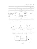
. We can simply graph
|R
3
(x)|on [0.3, 1.7], obtaining the graph shown in Figure 30.6. Using the tracer we estimate
that the magnitude of the error is less than 0.145.
As an exercise, use Taylor’s Remainder to estimate the error.
x
y
0.3 1.710.1

0.1
0.2
0.3
(.3, ≈ .14464)
Graph of |R
3
(x)| = ln x – (x–1) –
(x–1)
2
2
(x–1)
3
3
+
]
||
]
Figure 30.6
◆
EXAMPLE 30.9 Use graphical methods to find an upper bound for the error involved in using the tangent
line approximation 1 −
1
2
x to approximate
1
√
1+x
for |x| < 0.001.
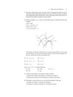
SOLUTION Graph R
2

(x) =(1 +x)
−
1
2
−

1 −
1
2
x

on the domain [−0.001, 001]. (Play around with the
range to obtain a useful graph.) The graph is given in Figure 30.7 on the following page.
938 CHAPTER 30 Series
3.8 × 10
–7
.001–.001
y
x
(–.001, ≈ 3.8 × 10
–7
) (.001, ≈ 3.8 × 10
–7
)
R
2
(x) = (1 + x) – [1 – x]
1
2
1

2
–
Figure 30.7
For |x| < 0.001, the approximation
1
√
1+x
≈ 1 −
1
2
x produces an error of less than
4 × 10
−7
.
◆
Any physicist will attest to the fact that physicists often use Taylor polynomials to
simplify mathematical expressions. In fact, they often use only first or second degree
polynomials. While this may at first strike you as a dubious strategy, the following example
will demonstrate that in certain situations the error introduced is minimal.
◆
EXAMPLE 30.10 According to Newtonian physics, an object’s kinetic energy, K,isgivenby
K=
1
2
m
0
v
2
,
where m

0
is the mass of the object at rest and v is its velocity.
Einstein’s theory of special relativity produces a more involved expression for K.
According to Einstein, the mass of an object is a function of its velocity, m =
m
0
√
1−v
2
/c
2
.
Einstein’s theory says energy, E, equals mc
2
, where c is the speed of light. He concludes
that an object’s kinetic energy is given by the difference mc
2
− m
0
c
2
. Using the expression
for m, Einstein’s theory says
K = m
0
c
2

1


1 − v
2
/c
2
− 1

= m
0
c
2




1 −
v
2
c
2

−
1
2
− 1



. (30.3)
Our goal in this example is to show that if an object is traveling much slower than the speed
of light, then according to Einstein’s theory, the error involved in using the Newtonian

expression for K is small.
SOLUTION We begin by noting that if v is substantially less than c, then
v
c
is small, and

v
c

2
is even
smaller. From Example 30.9 we know that (1 + x)
−
1
2
can be well approximated by its first
degree Taylor polynomial, 1 −
1
2
x, for |x| small. Let x =
−v
2
c
2
. Using the approximation

1 −
v
2
c

2

−
1
2
=

1 +

−
v
2
c
2

−
1
2
≈ 1 −
1
2

−
v
2
c
2

in Equation (30.3) we obtain
30.2 Error Analysis and Taylor’s Theorem 939

K = m
0
c
2




1 −
v
2
c
2

−
1
2
− 1



≈ m
0
c
2

1 +
1
2
v

2
c
2
− 1

= m
0
c
2
1
2
v
2
c
2
=
1
2
m
0
v
2
.
Let’s estimate the size of the error introduced by using the Newtonian expression for K for
an object traveling at speeds of 300 m/s or less. c = 3 · 10
8
m/s.
We’ ll find an upper bound for the error in replacing (1 + x)
−
1

2
by 1 −
1
2
x for |x|≤
300
2
c
2
and multiply the answer by m
0
c
2
.
|R
1
(x)|=
|f

(a)|
2!
|x|
2
for some a between 0 and 300.
f(x)=(1+x)
−
1
2
; f


(x) =−
1
2
(1 + x)
−
3
2
; f

(x) =
3
4
(1 + x)
−
5
2
|R
1
(x)|=
3
2 ·4(
√
1 + a)
5
x
2
≤
3
8



1 −
300
2
c
2

5
300
4
c
4
≈ 3.75 × 10
−25
Multiplying by m
0
c
2
gives m
0
3.375 × 10
−8
.
Therefore, for speeds of up to 300 m/s, the error incurred in computing K using
Newtonian physics is less than 3.4 × 10
−8
m
0
, where m
0

is the mass of the body at rest.
◆
PROBLEMS FOR SECTION 30.2
1. Find a good upper bound for the magnitude of the error involved in approximating
cos x by 1 −
x
2
2!
+
x
4
4!
for |x|≤0.2. Do this using Taylor’s Inequality; then check your
answer by graphing the remainder function.
2. Use the third degree Taylor polynomial for e
x
at x =0 to estimate
√
e. Then use Taylor’s
Theorem to get a reasonable upper bound for the remainder.
3. We will use the nth degree Taylor polynomial for e
x
,

n
k=0
x
k
k!
, to approximate

1
√
e
.
What should n be in order to guarantee that the approximation is off by less than 10
−5
?
4. Use the third degree Taylor polynomial for ln x centered at x = 1, (x − 1) −
(x−1)
2
2
+
(x−1)
3
3
, to approximate ln(1.5). Then give an upper bound for the remainder using
Taylor’s Theorem.
5. The second degree Taylor polynomial for f(x)=(1+x)
p
is 1 + px +
p(p−1)
2!
x
2
.If
the second degree Taylor polynomial is used to approximate
√
1 + x for |x|≤0.2, find
an upper bound for the magnitude of the error. Use the Taylor Inequality; then check
your answer by graphing R

2
(x).
940 CHAPTER 30 Series
6. For x near zero, cos x ≈1 −
x
2
2!
+
x
4
4!
− ···+(−1)
n
x
2n
(2n)!
. What degree Taylor polyno-
mial must be used to approximate cos(0.2) with error less than
1
10
8
?
7. Approximate
3
√
27.5 using an appropriate second degree Taylor polynomial. Find a
good upper bound for the error by using Taylor’s Inequality.
8. The second degree Taylor polynomial generated by ln(1 + x) about x = 0isx−
x
2

2
.
Use Taylor’s Theorem to find a good upper bound on the error involved in using this
polynomial to approximate the following.
(a) ln(1.2) (b) ln(0.8)
9. By graphing R
2
(x), estimate the values of x for which the approximation
ln x ≈ (x − 1) −
(x−1)
2
2!
can be used without producing an error of magnitude greater
than 10
−3
.
10. For x near zero, e
x
≈ 1 +x +
x
2
2!
+
x
3
3!
. Find a reasonable upper bound for the magni-
tude of the error involved in using this approximation for |x| < 0.5. Use Taylor’s
Inequality and check your answer by graphing R
3

(x).
11. A hyena is loping down a straight path away from a stream. The hyena is 6 m from the
stream, moving at a rate of 2 m/s and decelerating at a rate of 0.1 m/s
2
. Use a second
degree Taylor polynomial to estimate its distance from the stream 1 second later.
12. What degree Taylor polynomial for e
x
about x = 0 must be used to approximate e
0.3
with error less than 10
−5
?
13. (a) Find the nth degree Taylor polynomial for f(x)=
1
1−x
centered at x = 0.
(b) How many nonzero terms of the polynomial in part (a) must be used to approximate
f

1
2

with error less than 10
−5
?
14. According to Einstein’s theory of special relativity, the mass of an object moving with
velocity v m/s is given by
m =
m

0

1 −
v
2
c
2
,
where m
0
is the mass of the object at rest and c is the speed of light, c = 3 × 10
8
m/s.
(a) Use the first degree Taylor polynomial for
1
√
1+x
to arrive at the estimate
m ≈ m
0
+
m
0
2
v
2
c
2
.
(b) If an object is moving at 100 m/s, find an upper bound for the error involved in

using the approximation given in part (a).