Calculus: An Integrated Approach to Functions and their Rates of Change, Preliminary Edition Part 106 ppt

31.5 Systems of Differential Equations 1031
Where
dx
dt
= 0but
dy
dt
= 0, only y is changing with t so the trajectory’s tangent line is
vertical. The sign of
dy
dt
indicates how y changes with t; we display this information
by orienting the vertical tangents up or down.
Where
dy
dt
= 0but
dx
dt
= 0, only x is changing with t so the trajectory’s tangent line is
horizontal. The sign of
dx
dt
indicates how x changes with t; we display this information
by orienting the horizontal tangents right or left.
Where
dx
dt
= 0 and
dy
dt

= 0 simultaneously, the system is at equilibrium. Equilibrium
points are the points of intersection of nullclines for which
dx
dt
= 0 and those for which
dy
dt
= 0.
The nullclines partition the phase plane into regions in which neither
dx
dt
nor
dy
dt
changes
sign. In each region we’ll have one of the following cases:
dx
dt
> 0,
dy
dt
> 0

 
as t increases,
both x and y increase
dx
dt
> 0,
dy

dt
< 0

 
as t increases,
x increases and y decreases
dx
dt
< 0,
dy
dt
> 0

 
as t increases,
x decreases and y increases
dx
dt
< 0,
dy
dt
< 0

 
as t increases,
both x and y decrease
Sketch possible trajectories using the information gathered.
Fact The limit point of a trajectory must be an equilibrium point. By this we mean the
following. Suppose lim
t→∞

x(t) and lim
t→∞
y(t) both exist and are finite. Denote the
limits by A and B, respectively. Then (A, B) must be an equilibrium point. (Verify that
this is indeed the case in Examples 31.24 and 31.25.)
Note the analogy to the case of solutions to autonomous differential equations. If
y
1
(t) is a solution to an autonomous equation and lim
t→∞
y
1
(t) = L, where L is finite,
then y(t) = L is an equilibrium solution.
The slope of a trajectory at any point is
dy
dx
=
dy/dt
dx/dt
=
g(x,y)
f(x,y)
evaluated at that point
(provided f(x,y) = 0). Sometimes explicitly solving for a relationship between x and
y is enlightening.
◆
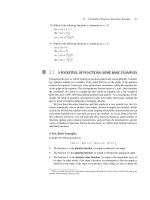
EXAMPLE 31.26 Analyze the following system of differential equations, sketching solution trajectories in
the xy-plane.


dx
dt
= y
dy
dt
=−x
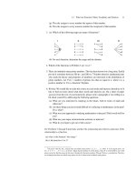
SOLUTION We begin by finding the nullclines.
The trajectories are horizontal where
dy
dt
=−x=0,i.e., along the y-axis.
The trajectories are vertical where
dx
dt
= y = 0, i.e., along the x-axis.
We can figure out the direction in which the trajectories are traveled along the nullclines by
looking back at the original equations. For example,
dx
dt
= y, so on the part of the y-axis
with y>0weknow
dx
dt
> 0; the trajectories are traveled from left to right, x increasing
with t. On the section of the y-axis with y<0,
dx
dt
< 0 so the trajectories are traveled from
1032 CHAPTER 31 Differential Equations
right to left, x decreasing with t. Vertical and horizontal tangents are oriented as shown in

Figure 31.23.
The only equilibrium point is the origin.
y
x
II I
III IV
Figure 31.23
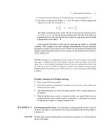
The nullclines partition the plane into the four regions labeled. In each region we look
at the signs of
dy
dt
and
dx
dt
to determine the basic direction of the trajectory.
Region I:
dx
dt
= y>0

 
x increases
,
dy
dt
=−x<0

 
y decreases
Region III:

dx
dt
= y<0

 
x decreases
,
dy
dt
=−x>0

 
y increases
Region II:
dx
dt
= y>0

 
x increases
,
dy
dt
=−x>0

 
y increases
Region IV:
dx
dt

= y<0

 
x decreases
,
dy
dt
=−x<0

 
y decreases
This information is collected in Figure 31.24.
y
x
II I
III IV
Figure 31.24
At this point we have some idea of what the trajectories look like. However, we are not
sure, for instance, if they form closed circles, or ellipses, or if they spiral in or spiral out.
We can look at
dy
dx
and try to solve the resulting differential equation to uncover the shapes
of the trajectories.
dy
dx
=
dy
dt
dx

dt
=
−x
y
, y = 0
so
31.5 Systems of Differential Equations 1033
dy
dx
=
−x
y
.
Separate variables and solve.
ydy=−xdx

ydy=

−xdx
y
2
2
=−
x
2
2
+ C
1
⇒ x
2

+ y
2
= C
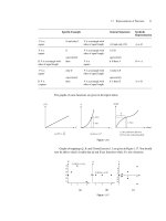
Therefore, the trajectories in the xy-plane are circles centered at the origin; the picture in
the phase plane is given in Figure 31.25.
y
x
Figure 31.25
Through every point in the xy-plane there is one trajectory passing through that point. Each
trajectory is a circle, except for the origin, which can be thought of as a degenerate circle
with radius 0. As t increases, the point (x(t), y(t)) traces out a circle in the clockwise
direction.
◆
REMARK The system of equations in Example 31.26 can arise when modeling the vibrations
of a frictionless spring. Consider a spring and attached block positioned as shown in Figure
31.26. Let x give the position of the block (of negligible weight) attached to the end of the
spring. Suppose we stretch the spring by pulling the block from its original position (x = 0)
out to x
0
and release the block.
x
0
x = 0
Figure 31.26
The block will oscillate back and forth about x = 0 and, in the absence of friction, will
repeat its motion ad infinitum. We expect the graph of x versus t to look like Figure 31.27
on the following page.
1034 CHAPTER 31 Differential Equations
x
0

x
t
Figure 31.27
Let y = the velocity of the block. Then y =
dx
dt
; velocity is the derivative of position
with respect to time. By Newton’s second law we know that force = (mass) · (acceleration).
We can denote the mass of the block by m and its acceleration by
d
2
x
dt
2
or
dy
dt
. Hooke’slaw,an
experimentally derived law, tells us that the force exerted by the spring is proportional to the
displacement from its equilibrium length. Putting the two laws together gives −∝x=m
dy
dt
or
dy
dt
=−kx for some k>0.Acceleration,
dy
dt
, is proportional to x but opposite in sign.
The proportionality constant is determined by the mass of the block and the nature of the

spring. (Think through some special cases to assure yourself that the equation
dy
dt
=−kx
makes sense in terms of the spring.) The frictionless block and spring system can therefore
be modeled by the system of differential equations

dx
dt
= y
dy
dt
=−kx.
For convenience let’s assume that k = 1. Then the equations describing the motion become
dx
dt
= y and
dy
dt
=−x.
Look back at the phase-plane diagram (Figure 31.25) to see how the motion of the
spring is reflected in this picture. If we pull the block out a distance x
0
and simply let it go,
giving it no initial velocity, we should look at the point (x
0
,0)in the phase plane. Follow
the trajectory around in the direction of the arrow and note how the position of the block
(the x-coordinate) and the velocity of the block (the y-coordinate) change with time.
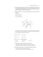
EXERCISE 31.8 It is unrealistic to ignore friction. Let x(t) be the position of the block.


x(0) = x
0
x

(0) = 0
(a) Sketch a possible graph of x versus t for the spring example, considering the force of
friction and assuming the block vibrates back and forth several times.
(b) Now, letting y =
dx
dt
= velocity, sketch the trajectory in the xy-plane. (In the next section
we will deal analytically with the friction issue.)
The answer to Exercise 31.8 appears at the end of the section.
Returning to Epidemic Model B: A Contagious, Fatal Disease
◆
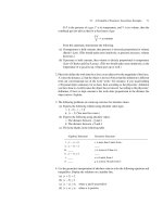
EXAMPLE 31.27 Consider the epidemic model that was used to motivate this discussion. Residing in a large
susceptible population is a small group of people with a fatal infectious disease. An infected
31.5 Systems of Differential Equations 1035
individual can immediately infect others, and any person not infected is susceptible. We
make the assumption that the population remains fixed during the time interval in question
except for deaths due to the disease. I (t ) = the number of infected people at time t, and
S(t) = the number of susceptible people at time t.
dS
dt
=−rSI, where r>0
As the susceptible class loses members, the infected class gains members but it also loses
people due to death from the disease.
dI
dt

= rSI − kI, where r, k>0
Analyze the system of equations

dS
dt
=−rSI
dI
dt
= I (rS − k) r, k>0, sketching solution trajectories in the SI-plane.
SOLUTION Look for the nullclines and equilibrium points. Let’s plot S on the horizontal axis and I on
the vertical axis. Then the slopes of the trajectories are given by
dI
dS
=
dI/dt
dS/dt
.
The trajectories are horizontal where
dI
dt
= I (rS − k) = 0, that is, for I = 0orS=
k
r
.
The trajectories are vertical where
dS
dt
=−rSI = 0, that is, for S = 0orI=0.
The system is at equilibrium if and only if
dI

dt
= 0 and
dS
dt
= 0 simultaneously. S cannot
simultaneously be 0 and
k
r
, so the equilibria for the system are at I = 0. Every point
on the S-axis is an equilibrium point.
The nullclines are S = 0, I = 0, and S =
k
r
. These partition the first quadrant into two
regions, I and II, as indicated in Figure 31.28.
I
S
II I
k
r
Figure 31.28
Region I Region II
sign of
dS
dt
: −−
sign of
dI
dt
: +−

Weknow that the solution curves go in the direction of the arrows drawn in Figure 31.28.
Further information about the shape of the trajectories in the SI-plane can be obtained by
looking at
dI
dS
.
dI
dS
=
dI/dt
dS/dt
=
I (rS − k)
−rSI
=
rS − k
−rS
=−1+
k
rS
.
1036 CHAPTER 31 Differential Equations
The slope is a function of S; the trajectories are vertical translates. (As an exercise, solve
for I in terms of S.) The second derivative of I with respect to S is given by
d
2
I
dS
2
=−

k
rS
2
,
where r and k are positive constants.
d
2
I
dS
2
< 0, so the trajectories are concave down. See
Figure 31.29.
(S
0
, I
0
)
I
S
k
r
Figure 31.29
REMARKS Observe that if S
0
<
k
r
, then I immediately decreases toward zero; the disease
leaves the population without becoming an epidemic. On the other hand, if S
0

>
k
r
, then the
disease will spread and the number of infected people will increase until S drops to
k
r
. Only
when S falls below the threshold value of
k
r
does I begin to decrease. The disease does not
die out completely for lack of a susceptible population but rather for lack of infected people.
Generally, some individuals will remain who have not caught the disease.
◆
The same system of differential equations that were set up in the previous example can
also be used to model an epidemic such as measles or chicken pox, where instead of the
disease being fatal, sickness confers immunity upon those who recover. Once an individual
is infected he cannot become reinfected, so after leaving the “infected” class he does not
rejoin the “susceptible” class but belongs to a “recovered” class.
◆
EXAMPLE 31.28 In an isolated community of 800 susceptible children, one child is diagnosed with chicken
pox. Suppose the spread of the disease can be modeled by the system of differential
equations

dS
dt
=−0.001SI
dI
dt

= 0.001SI − 0.3I .
(a) What is the maximum number of children sick at any one moment?
(b) According to our model, how many susceptible children will avoid getting chicken pox
while the epidemic runs its course?
SOLUTION (a) From the qualitative analysis done in Example 31.27 we know that I is maximum
when S =
k
r
, that is, when
dI
dS
= 0. So I is maximum at S =
0.3
.001
= 300. To find I when
S = 300 we need an explicit relationship between I and S. I = 800 − S because some
infected children have already recovered.
dI
dS
=
dI/dt
dS/dt
=
0.001SI − 0.3I
−0.001SI
=−1+
0.3
0.001S
=−1+
300

S
31.5 Systems of Differential Equations 1037
Separate variables and integrate to obtain I as a function of S.
dI =

−1 +
300
S

dS

dI =

(−1)dS + 300

dS
S
I =−S+300 ln S + C, S>0, so |S|=S.
Use the initial conditions, I = 1 and S = 800 when t = 0, to solve for C.
1 =−800 + 300 ln(800) + C,soC=801 − 300 ln(800) ≈−1204.38
Then
I (S) ≈−S+300 ln S − 1204, and
I(300) ≈−300 + 300 ln 300 − 1204 ≈ 207.
There were at most about 207 children sick at one time. This is just over a quarter of
the susceptible population.
(b) As pointed out in Example 31.27, the epidemic ends not for lack of susceptible children
but for lack of infected children. Therefore, we set I = 0 and solve for S. Because
the equation involves both S and ln S we can only approximate the solution. Using
a calculator, computer, or numerical methods, we find that S ≈ 70. At the end of the
epidemic about 70 children will still be susceptible to chicken pox; 730 children will

have caught the disease.
◆
In some sense, in the previous two examples it is the ratio
k
r
that governs the course
of the epidemic. The likelihood of the disease being passed from one individual to the
next is reflected in r. For a disease such as chicken pox, communities sometimes attempt
to raise the value of r (to confer immunity before adulthood) whereas for a fatal infectious
disease, like AIDs, communities sometimes educate to lower the value of r. When dangerous
epidemics break out in livestock populations, farmers and ranchers often remove sick
animals, effectively raising the value of k, in order to end up with more uninfected animals.
Recurrent Epidemics
Many diseases recur in various populations with some regularity. For instance, in London
in the early 1900s, measles epidemics recurred approximately every two years. In 1929,
when the mathematical biologist H. E. Soper was attempting to model this cyclic measles
epidemic, he dropped the assumption that the population remains fixed for the time interval
being observed. Instead he assumed that the population of susceptibles grows at a constant
rate µ and arrived at this system of differential equations:
dS
dt
=−rSI + µ
dI
dt
= rSI − kI for r, k, and µ positive constants
In fact this system of equations does not predict recurrent outbreaks of the epidemic. Instead
it predicts that the disease will reach a steady state level since the cycles are heavily damped.
The problem with this model is the assumption that the susceptible population grows at a
constant rate. Try to modify this system of equations. If you assume the population grows at
1038 CHAPTER 31 Differential Equations

a rate proportional to itself, then the solutions to the equations are cyclic and undamped, as
desired. Think about the repeating cycle of measles epidemics again after working through
Example 31.29.
Modeling Population Interactions
The more closely we look at the world the more clearly we see its interconnected nature.
We can use the tools we’ve developed in this section to model interactions between distinct
populations. We can model symbiotic interactions, such as the interaction between sea
anemones and clown fish, or competitive interactions, such as the interaction between lion
and hyena populations competing for small prey. We can model predator-prey interactions,
such as that between hyenas and the Thomson’s gazelle, lions and water buffalo, or cats
and mice. In the examples in this section we’ll simplify our models to focus on just two
populations.
◆
EXAMPLE 31.29 Consider the predator-prey relationship between hyenas and the Thomson’s gazelle, a small
gazelle native to Africa. Let’s make the following simplifying assumptions.
i. Assume hyenas are the gazelles’ major predator and that in the hyenas’ absence the
gazelle population would grow exponentially.
ii. Assume gazelles are the major food source for hyenas; with no gazelles the hyenas
would die off.
Model this interaction with a system of differential equations.
SOLUTION Let h(t) = the number of hundreds of hyenas at time t.
Let g(t) = the number of hundreds of gazelles at time t.
We can model the interaction by a system of differential equations of the form

dh
dt
=−k
1
h+k
2

hg
dg
dt
= k
3
g − k
4
hg
where k
1
, k
2
, k
3
, and k
4
are positive constants. Just as the rate of transmission of disease
is proportional to interactions between the infected and the susceptible, which is in turn
proportional to the product of their numbers, so too is the rate of nourishing/fatal interaction
between hyena and gazelle proportional to the product of their population sizes. Observe
that if h = 0 then
dg
dt
= k
3
g and if g = 0 then
dh
dt
=−k
1

h.For the sake of concreteness, we’ll
work with the values of k
1
, k
2
, k
3
, and k
4
given below and analyze solutions in the gh-plane.
dh
dt
=−0.3h + 0.1gh = 0.1h(−3 + g)
dg
dt
=+0.4g − 0.4gh = 0.4g(1 − h)
Nullclines:
dh
dt
= 0 when h = 0org=3. In the gh-plane this is where trajectories have
horizontal tangent lines.
dg
dt
= 0 when g = 0orh=1. In the gh-plane this is where trajectories have vertical
tangent lines.
Equilibrium points:
dh
dt
= 0ath=0org=3, so at an equilibrium point either h = 0or
g=3.

31.5 Systems of Differential Equations 1039
Suppose h = 0. Then in order for
dg
dt
to be zero we must have g = 0. (0, 0) is an
equilibrium point.
Suppose g = 3. Then in order for
dg
dt
to be zero we must have h = 1. The point (3, 1)
is an equilibrium point.
Use the differential equations to orient the vertical and horizontal tangents. For instance,
when g = 3 we know that
dg
dt
> 0 for 0 <h<1and
dg
dt
< 0 for h>1.
h
g
1
3
Figure 31.30
The h and g axes are oriented as shown in Figure 31.30. The nullclines divide the relevant
first quadrant region into four subregions. The direction of trajectories in each region is
indicated in Figure 31.30.
From Figure 31.30 we see that for g(0)>0and h(0)>0the trajectories either spiral
in toward (3, 1) or spiral outward, or are closed curves. From the slope field it appears that
the curves are closed. Looking at

dh
dg
=
0.1h(−3+0.1g)
0.4g(1−h)
enables us to distinguish between these
options. Separating variables, we find that
ln(h) − h =−3ln(g) + g + C.
Suppose we start at the point (5, 1). We can solve for C and show that the trajectory through
(5, 1) intersects the line g = 3 exactly twice, once for h>1and once for h<1. Similarly
we can show that it intersects the line h = 1 exactly twice, once for g<3and once for
g>3. The trajectory through (5, 1) is a closed curve. In fact, all the trajectories in the first
quadrant are closed.
g
h
3
1
Figure 31.31
Our model predicts that the hyena and gazelle populations will oscillate cyclically.
When there are few gazelle the hyena population decreases due to lack of food. The decrease
1040 CHAPTER 31 Differential Equations
in the number of hyenas allows the gazelle population to thrive, but as the gazelle population
increases the hyenas’ food source is replenished, allowing the hyena population to flourish.
This flourishing takes its toll on the gazelles, and the cycle repeats. ◆
To the extent that a model reflects observed population dynamics, it is a good model.
Models that don’treflect observed behavior must be modified. There are various ways this
predator-prey model can be modified. For instance, there may be competition among gazelle
for limited grazing land so that in the absence of hyena the gazelle population exhibits
logistic growth. This can be reflected in the system of differential equations by inserting a
−k

5
g
2
term as shown.

dh
dt
=−k
1
h+k
2
hg
dg
dt
= k
3
g − k
4
hg − k
5
g
2
,
where the −k
5
g
2
term (k
5
> 0) reflects competition among gazelles.

The predator-prey system of differential equations given in Example 31.29 is sometimes
referred to as Volterra’s model after the Italian mathematician Vito Volterra (1860-1940)
who was encouraged to analyze the predator-prey relationship between sharks and the
fish they prey upon by his son-in-law, the biologist Humberto D’Ancona.
10
By inserting
a term in each equation to account for fishing, Volterra was able to explain why fishing
conducted in the Adriatic Sea was raising the average number of prey and lowering the
average number of predators over any cycle. Similar analysis has been successfully used
to analyze unexpected results of introducing DDT into a predator-prey system, leaving
predator populations lowered and prey populations elevated.
Competition between species can be modeled by differential equations of the form

dx
dt
= k
1
x − k
2
xy
dy
dt
= k
4
y − k
5
xy
or

dx

dt
= k
1
x − k
2
xy − k
3
x
2
dy
dt
= k
4
y − k
5
xy − k
6
y
2
where k
1
, k
2
, ,k
6
are positive constants. The latter set of differential equations takes
into account competition between members of the same species in addition to competition
between species.
Answers to Selected Exercises
Answers to Exercise 31.8

x
x
y(b)(a)
x
0
x
0
t
10
For more information on a very interesting story see Martin Braun, Differential Equations and their Applications, 2nd ed.
New York. Springer Verlag, 1978 or G. F. Gause, The Struggle for Existence, New York. Hafner, 1964, or Umberto D’Ancona,
The Struggle for Existence, Leiden, Brill, 1954.