Quantitative Models in Marketing Research Chapter 3 pdf
Bạn đang xem bản rút gọn của tài liệu. Xem và tải ngay bản đầy đủ của tài liệu tại đây (247.89 KB, 20 trang )
3 A continuous dependent variable
In this chapter we review a few principles of econometric modeling, and
illustrate these for the case of a continuous dependent variable. We assume
basic knowledge of matrix algebra and of basic statistics and mathematics
(differential algebra and integral calculus). As a courtesy to the reader, we
include some of the principles on matrices in the Appendix (section A.1).
This chapter serves to review a few issues which should be useful for later
chapters. In section 3.1 we discuss the representation of the standard Linear
Regression model. In section 3.2 we discuss Ordinary Least Squares and
Maximum Likelihood estimation in substantial detail. Even though the
Maximum Likelihood method is not illustrated in detail, its basic aspects
will be outlined as we need it in later chapters. In section 3.3, diagnostic
measures for outliers, residual autocorrelation and heteroskedasticity are
considered. Model selection concerns the selection of relevant variables
and the comparison of non-nested models using certain model selection
criteria. Forecasting deals with within-sample or out-of-sample prediction.
In section 3.4 we illustrate several issues for a regression model that corre-
lates sales with price and promotional activities. Finally, in section 3.5 we
discuss extensions to multiple-equation models, thereby mainly focusing on
modeling market shares.
This chapter is not at all intended to give a detailed account of econo-
metric methods and econometric analysis. Much more detail can, for
example, be found in Greene (2000), Verbeek (2000) and Wooldridge
(2000). In fact, this chapter mainly aims to set some notation and to highlight
some important topics in econometric modeling. In later chapters we will
frequently make use of these concepts.
3.1 The standard Linear Regression model
In empirical marketing research one often aims to correlate a ran-
dom variable Y
t
with one (or more) explanatory variables such as x
t
, where
29
30 Quantitative models in marketing research
the index t denotes that these variables are measured over time, that is,
t ¼ 1; 2; ; T. This type of observation is usually called time series observa-
tion. One may also encounter cross-sectional data, which concern, for
example, individuals i ¼ 1; 2; ; N, or a combination of both types of
data. Typical store-level scanners generate data on Y
t
, which might be the
weekly sales (in dollars) of a certain product or brand, and on x
t
, denoting
for example the average actual price in that particular week.
When Y
t
is a continuous variable such as dollar sales, and when it seems
reasonable to assume that it is independent of changes in price, one may
consider summarizing these sales by
Y
t
$ Nð;
2
Þ; ð3:1Þ
that is, the random variable sales is normally distributed with mean and
variance
2
. For further reference, in the Appendix (section A.2) we collect
various aspects of this and other distributions. In figure 3.1 we depict an
example of such a normal distribution, where we set at 1 and
2
at 1. In
practice, the values of and
2
are unknown, but they could be estimated
from the data.
In many cases, however, one may expect that marketing instruments such
as prices, advertising and promotions do have an impact on sales. In the case
of a single price variable, x
t
, one can then choose to replace (3.1) by
Y
t
$ Nð
0
þ
1
x
t
;
2
Þ; ð3:2Þ
0.0
0.1
0.2
0.3
0.4
0.5
_
4
_
2
0 2 4
Figure 3.1 Density function of a normal distribution with ¼
2
¼ 1
A continuous dependent variable 31
where the value of the mean is now made dependent on the value of the
explanatory variable, or, in other words, where the conditional mean of Y
t
is
now a linear function of
0
and
1
x
t
, with
0
and
1
being unknown para-
meters. In figure 3.2, we depict a set of simulated y
t
and x
t
, generated by
x
t
¼ 0:0001t þ"
1;t
with "
1;t
$ Nð0; 1Þ
y
t
¼À2 þ x
t
þ "
2;t
with "
2;t
$ Nð0; 1Þ;
ð3:3Þ
where t is 1; 2; ; T. In this graph, we also depict three density functions of
a normal distribution for three observations on Y
t
. This visualizes that each
observation on y
t
equals
0
þ
1
x
t
plus a random error term, which in turn is
a drawing from a normal distribution. Notice that in many cases it is unlikely
that the conditional mean of Y
t
is equal to
1
x
t
only, as in that case the line
in figure 3.2 would always go through the origin, and hence one should better
always retain an intercept parameter
0
.
In case there is more than one variable having an effect on Y
t
, one may
consider
Y
t
$ Nð
0
þ
1
x
1;t
þÁÁÁþ
K
x
K;t
;
2
Þ; ð3:4Þ
where x
1;t
to x
K;t
denote the K potentially useful explanatory variables. In
case of sales, variable x
1;t
can for example be price, variable x
2;t
can be
advertising and variable x
3;t
can be a variable measuring promotion. To
simplify notation (see also section A.1 in the Appendix), one usually defines
_
8
_
6
_
4
_
2
0
2
4
_
4
_
2
0 2 4
x
t
y
t
Figure 3.2 Scatter diagram of y
t
against x
t
32 Quantitative models in marketing research
the ðK þ1ÞÂ1 vector of parameters , containing the K þ1 unknown para-
meters
0
,
1
to
K
, and the 1 ÂðK þ1Þ vector X
t
, containing the known
variables 1, x
1;t
to x
K;t
. With this notation, (3.4) can be summarized as
Y
t
$ NðX
t
;
2
Þ: ð3:5Þ
Usually one encounters this model in the form
Y
t
¼ X
t
þ "
t
; ð3:6Þ
where "
t
is an unobserved stochastic variable assumed to be distributed as
normal with mean zero and variance
2
, or in short,
"
t
$ Nð0;
2
Þ: ð3:7Þ
This "
t
is often called an error or disturbance. The model with components
(3.6) and (3.7) is called the standard Linear Regression model, and it will be
the focus of this chapter.
The Linear Regression model can be used to examine the contempora-
neous correlations between the dependent variable Y
t
and the explanatory
variables summarized in X
t
. If one wants to examine correlations with pre-
viously observed variables, such as in the week before, one can consider
replacing X
t
by, for example, X
tÀ1
. A parameter
k
measures the partial
effect of a variable x
k;t
on Y
t
, k 2f1; 2; ; Kg, assuming that this variable
is uncorrelated with the other explanatory variables and "
t
. This can be seen
from the partial derivative
@Y
t
@x
k;t
¼
k
: ð3:8Þ
Note that if x
k;t
is not uncorrelated with some other variable x
l;t
, this
partial effect will also depend on the partial derivative of x
l;t
to x
k;t
, and
the corresponding
l
parameter. Given (3.8), the elasticity of x
k;t
for y
t
is
now given by
k
x
k;t
=y
t
. If one wants a model with time-invariant elasticities
with value , one should consider the regression model
log Y
t
$ Nð
0
þ
1
log x
1;t
þÁÁÁþ
K
log x
K;t
;
2
Þ; ð3:9Þ
where log denotes the natural logarithmic transformation, because in that
case
@Y
t
@x
k;t
¼
k
y
t
x
k;t
: ð3:10Þ
Of course, this logarithmic transformation can be applied only to positive-
valued observations. For example, when a 0/1 dummy variable is included to
measure promotions, this transformation cannot be applied. In that case,
A continuous dependent variable 33
one simply considers the 0/1 dummy variable. The elasticity of such a
dummy variable then equals expð
k
ÞÀ1.
Often one is interested in quantifying the effects of explanatory variables
on the variable to be explained. Usually, one knows which variable should be
explained, but in many cases it is unknown which explanatory variables are
relevant, that is, which variables appear on the right-hand side of (3.6). For
example, it may be that sales are correlated with price and advertising, but
that they are not correlated with display or feature promotion. In fact, it is
quite common that this is exactly what one aims to find out with the model.
In order to answer the question about which variables are relevant, one
needs to have estimates of the unknown parameters, and one also needs to
know whether these unknown parameters are perhaps equal to zero. Two
familiar estimation methods for the unknown parameters will be discussed in
the next section.
Several estimation methods require that the maintained model is not mis-
specified. Unfortunately, most models constructed as a first attempt are
misspecified. Misspecification usually concerns the notion that the main-
tained assumptions for the unobserved error variable "
t
in (3.7) are violated
or that the functional form (which is obviously linear in the standard Linear
Regression model) is inappropriate. For example, the error variable may
have a variance which varies with a certain variable, that is,
2
is not con-
stant but is
2
t
, or the errors at time t are correlated with those at t À 1, for
example, "
t
¼ "
tÀ1
þ u
t
. In the last case, it would have been better to include
y
tÀ1
and perhaps also X
tÀ1
in (3.5). Additionally, with regard to the func-
tional form, it may be that one should include quadratic terms such as x
2
k;t
instead of the linear variables.
Unfortunately, usually one can find out whether a model is misspecified
only once the parameters for a first-guess model have been estimated. This is
because one can only estimate the error variable given these estimates, that is
^
""
t
¼ y
t
À X
t
^
; ð3:11Þ
where a hat indicates an estimated value. The estimated error variables are
called residuals. Hence, a typical empirical modeling strategy is, first, to put
forward a tentative model, second, to estimate the values of the unknown
parameters, third, to investigate the quality of the model by applying a
variety of diagnostic measures for the model and for the estimated error
variable, fourth, to re-specify the model if so indicated by these diagnostics
until the model has become satisfactory, and, finally, to interpret the values
of the parameters. Admittedly, a successful application of this strategy
requires quite some skill and experience, and there seem to be no straightfor-
ward guidelines to be followed.
34 Quantitative models in marketing research
3.2 Estimation
In this section we briefly discuss parameter estimation in the stan-
dard Linear Regression model. We first discuss the Ordinary Least Squares
(OLS) method, and then we discuss the Maximum Likelihood (ML) method.
In doing so, we rely on some basic results in matrix algebra, summarized in
the Appendix (section A.1). The ML method will also be used in later chap-
ters as it is particularly useful for nonlinear models. For the standard Linear
Regression model it turns out that the OLS and ML methods give the same
results. As indicated earlier, the reader who is interested in this and the next
section is assumed to have some prior econometric knowledge.
3.2.1 Estimation by Ordinary Least Squares
Consider again the standard Linear Regression
model
Y
t
¼ X
t
þ "
t
; with "
t
$ Nð0;
2
Þ: ð3:12Þ
The least-squares method aims at finding that value of for which
P
T
t¼1
"
2
t
¼
P
T
t¼1
ðy
t
À X
t
Þ
2
gets minimized. To obtain the OLS estimator we differenti-
ate
P
T
t¼1
"
2
t
with respect to and solve the following first-order conditions
for
@
X
T
t¼1
ðy
t
À X
t
Þ
2
@
¼
X
T
t¼1
X
0
t
ðy
t
À X
t
Þ¼0; ð3:13Þ
which yields
^
¼
X
T
t¼1
X
0
t
X
t
!
À1
P
T
t¼1
X
0
t
y
t
: ð3:14Þ
Under the assumption that the variables in X
t
are uncorrelated with the error
variable "
t
, in addition to the assumption that the model is appropriately
specified, the OLS estimator is what is called consistent. Loosely speaking,
this means that when one increases the sample size T, that is, if one collects
more observations on y
t
and X
t
, one will estimate the underlying with
increasing precision.
In order to examine if one or more of the elements of are equal to zero
or not, one can use
^
$
a
N ;
^
2
X
T
t¼1
X
0
t
X
t
!
À1
1
A
;
0
@
ð3:15Þ
A continuous dependent variable 35
where $
a
denotes ‘‘distributed asymptotically as’’, and where
^
2
¼
1
T ÀðK þ 1Þ
X
T
t¼1
ðy
t
À X
t
^
Þ
2
¼
1
T ÀðK þ 1Þ
X
T
t¼1
^
""
2
t
ð3:16Þ
is a consistent estimator of
2
. An important requirement for this result is
that the matrix ð
P
T
t¼1
X
0
t
X
t
Þ=T approximates a constant value as T increases.
Using (3.15), one can construct confidence intervals for the K þ1 parameters
in . Typical confidence intervals cover 95% or 90% of the asymptotic
distribution of
^
. If these intervals include the value of zero, one says that
the underlying but unknown parameter is not significantly different from
zero at the 5% or 10% significance level, respectively. This investigation is
usually performed using a so-called z-test statistic, which is defined as
z
^
k
¼
^
k
À 0
ffiffiffiffiffiffiffiffiffiffiffiffiffiffiffiffiffiffiffiffiffiffiffiffiffiffiffiffiffiffiffiffiffiffiffiffiffiffiffiffiffiffiffiffiffiffiffi
^
2
P
T
t¼1
X
0
t
X
t
À1
k;k
s
; ð3:17Þ
where the subscript (k; k) denotes the matrix element in the k’th row and k’th
column. Given the adequacy of the model and given the validity of the null
hypothesis that
k
¼ 0, it holds that
z
^
k
$
a
Nð0; 1Þ: ð3:18Þ
When z
^
k
takes a value outside the region ½À1:96; 1:96, it is said that the
corresponding parameter is significantly different from 0 at the 5% level (see
section A.3 in the Appendix for some critical values). In a similar manner,
one can test whether
k
equals, for example,
Ã
k
. In that case one has to
replace the denominator of (3.17) by
^
k
À
Ã
k
. Under the null hypothesis
that
k
¼
Ã
k
the z-statistic is again asymptotically normally distributed.
3.2.2 Estimation by Maximum Likelihood
An estimation method based on least-squares is easy to apply, and
it is particularly useful for the standard Linear Regression model. However,
for more complicated models, such as those that will be discussed in subse-
quent chapters, it may not always lead to the best possible parameter esti-
mates. In that case, it would be better to use the Maximum Likelihood (ML)
method.
In order to apply the ML method, one should write a model in terms of
the joint probability density function pðyjX; Þ for the observed variables y
given X, where summarizes the model parameters and
2
, and where p
36 Quantitative models in marketing research
denotes probability. For given values of , pðÁjÁ; Þ is a probability density
function for y conditional on X. Given ðyjXÞ, the likelihood function is
defined as
LðÞ¼pðyjX; Þ: ð3:19Þ
This likelihood function measures the probability of observing the data ðyjXÞ
for different values of . The ML estimator
^
is defined as the value of that
maximizes the function LðÞ over a set of relevant parameter values of .
Obviously, the ML method is optimal in the sense that it yields the value of
^
that gives the maximum likely correlation between y and X, given X.
Usually, one considers the logarithm of the likelihood function, which is
called the log-likelihood function
lðÞ¼logðLðÞÞ: ð3:20Þ
Because the natural logarithm is a monotonically increasing transformation,
the maxima of (3.19) and (3.20) are naturally obtained for the same values
of .
To obtain the value of that maximizes the likelihood function, one first
differentiates the log-likelihood function (3.20) with respect to . Next, one
solves the first-order conditions given by
@lðÞ
@
¼ 0 ð3:21Þ
for resulting in the ML estimate denoted by
^
. In general it is usually not
possible to find an analytical solution to (3.21). In that case, one has to use
numerical optimization techniques to find the ML estimate. In this book we
opt for the Newton–Raphson method because the special structure of the
log-likelihood function of many of the models reviewed in the following
chapters results in efficient optimization, but other optimization methods
such as the BHHH method of Berndt et al. (1974) can be used instead
(see, for example, Judge et al., 1985, Appendix B, for an overview). The
Newton–Raphson method is based on meeting the first-order condition for
a maximum in an iterative manner. Denote the gradient GðÞ and Hessian
matrix HðÞ by
Gð Þ¼
@lðÞ
@
HðÞ¼
@
2
lðÞ
@@
0
;
ð3:22Þ
then around a given value
h
the first-order condition for the optimization
problem can be linearized, resulting in Gð
h
ÞþHð
h
Þð À
h
Þ¼0. Solving
this for gives the sequence of estimates
A continuous dependent variable 37
hþ1
¼
h
À Hð
h
Þ
À1
Gð
h
Þ: ð3:23Þ
Under certain regularity conditions, which concern the log-likelihood func-
tion, these iterations converge to a local maximum of (3.20). Whether a
global maximum is found depends on the form of the function and on the
procedure to determine the initial estimates
0
. In practice it can thus be
useful to vary the initial estimates and to compare the corresponding log-
likelihood values. ML estimators have asymptotically optimal statistical
properties under fairly mild conditions. Apart from regularity conditions
on the log-likelihood function, the main condition is that the model is ade-
quately specified.
In many cases, it holds true that
ffiffiffiffi
T
p
ð
^
À Þ$
a
Nð0;
^
II
À1
Þ; ð3:24Þ
where
^
II is the so-called information matrix evaluated at
^
, that is,
^
II¼ÀE
@
2
lðÞ
@@
0
"#
¼
^
; ð3:25Þ
where E denotes the expectation operator.
To illustrate the ML estimation method, consider again the standard
Linear Regression model given in (3.12). The log-likelihood function for
this model is given by
Lð;
2
Þ¼
Y
T
t¼1
1
ffiffiffiffiffiffi
2
p
expðÀ
1
2
2
ðy
t
À X
t
Þ
2
Þð3:26Þ
such that the log-likelihood reads
lð;
2
Þ¼
X
T
t¼1
À
1
2
log 2 À log À
1
2
2
ðy
t
À X
t
Þ
2
; ð3:27Þ
where we have used some of the results summarized in section A.2 of the
Appendix. The ML estimates are obtained from the first-order conditions
@lð;
2
Þ
@
¼
X
T
t¼1
1
2
X
0
t
ðy
t
À X
t
Þ¼0
@lð;
2
Þ
@
2
¼
X
T
t¼1
À
1
2
2
þ
1
2
4
ðy
t
À X
t
Þ
2
¼ 0:
ð3:28Þ
38 Quantitative models in marketing research
Solving this results in
^
¼
X
T
t¼1
X
0
t
X
t
!
À1
X
T
t¼1
X
0
t
y
t
^
2
¼
1
T
X
T
t¼1
ðy
t
À X
t
^
Þ
2
¼
1
T
X
T
t¼1
^
""
2
t
:
ð3:29Þ
This shows that the ML estimator for is equal to the OLS estimator in
(3.14), but that the ML estimator for
2
differs slightly from its OLS counter-
part in (3.16).
The second-order derivatives of the log-likelihood function, which are
needed in order to construct confidence intervals for the estimated para-
meters (see (3.24)), are given by
@
2
lð;
2
Þ
@@
0
¼À
1
2
X
T
t¼1
X
0
t
X
t
@
2
lð;
2
Þ
@@
2
¼À
1
4
X
T
t¼1
X
0
t
ðy
t
À X
t
Þ
@
2
lð;
2
Þ
@
2
@
2
¼
X
T
t¼1
1
2
4
À
1
6
ðy
t
À X
t
Þ
2
:
ð3:30Þ
Upon substituting the ML estimates in (3.24) and (3.25), one can derive that
^
$
a
N ;
^
2
X
T
t¼1
X
0
t
X
t
!
À1
0
@
1
A
; ð3:31Þ
which, owing to (3.29), is similar to the expression obtained for the OLS
method.
3.3 Diagnostics, model selection and forecasting
Once the parameters have been estimated, it is important to check
the adequacy of the model. If a model is incorrectly specified, there may be a
problem with the interpretation of the parameters. Also, it is likely that the
included parameters and their corresponding standard errors are calculated
incorrectly. Hence, it is better not to try to interpret and use a possibly
misspecified model, but first to check the adequacy of the model.
There are various ways to derive tests for the adequacy of a maintained
model. One way is to consider a general specification test, where the main-
tained model is the null hypothesis and the alternative model assumes that
A continuous dependent variable 39
any of the underlying assumptions are violated. Although these general tests
can be useful as a one-time check, they are less useful if the aim is to obtain
clearer indications as to how one might modify a possibly misspecified
model. In this section, we mainly discuss more specific diagnostic tests.
3.3.1 Diagnostics
There are various ways to derive tests for the adequacy of a main-
tained model. One builds on the Lagrange Multiplier (LM) principle. In
some cases the so-called Gauss–Newton regression is useful (see Davidson
and MacKinnon, 1993). Whatever the principle, a useful procedure is the
following. The model parameters are estimated and the residuals are saved.
Next, an alternative model is examined, which often leads to the suggestion
that certain variables were deleted from the initial model in the first place.
Tests based on auxiliary regressions, which involve the original variables and
the omitted variables, can suggest whether the maintained model should be
rejected for the alternative model. If so, one assumes the validity of the
alternative model, and one starts again with parameter estimation and diag-
nostics.
The null hypothesis in this testing strategy, at least in this chapter, is the
standard Linear Regression model, that is,
Y
t
¼ X
t
þ "
t
; ð3:32Þ
where "
t
obeys
"
t
$ Nð0;
2
Þ: ð3:33Þ
A first and important test in the case of time series variables (but not for
cross-sectional data) concerns the absence of correlation between "
t
and "
tÀ1
,
that is, the same variable lagged one period. Hence, there should be no
autocorrelation in the error variable. If there is such correlation, this can
also be visualized by plotting estimated "
t
against "
tÀ1
in a two-dimensional
scatter diagram. Under the alternative hypothesis, one may postulate that
"
t
¼ "
tÀ1
þ v
t
; ð3:34Þ
which is called a first-order autoregression (AR(1)) for "
t
. By writing
Y
tÀ1
¼ X
tÀ1
þ "
tÀ1
, and subtracting this from (3.32), the regression
model under this alternative hypothesis is now given by
Y
t
¼ Y
tÀ1
þ X
t
À X
tÀ1
þ v
t
: ð3:35Þ
It should be noticed that an unrestricted model with Y
tÀ1
and X
tÀ1
would
contain 1 þðK þ1ÞþK ¼ 2ðK þ1Þ parameters because there is only one
40 Quantitative models in marketing research
intercept, whereas, owing to the common parameter, (3.35) has only 1 þ
ðK þ1Þ¼K þ2 unrestricted parameters.
One obvious way to examine if the error variable "
t
is an AR(1) variable is
to add y
tÀ1
and X
tÀ1
to the initial regression model and to examine their joint
significance. Another way is to consider the auxiliary test regression
^
""
t
¼ X
t
þ
^
""
tÀ1
þ w
t
: ð3:36Þ
If the error variable is appropriately specified, this regression model should
not be able to describe the estimated errors well. A simple test is now given
by testing the significance of
^
""
tÀ1
in (3.36). This can be done straightfor-
wardly using the appropriate z-score statistic (see (3.17)). Consequently, a
test for residual autocorrelation at lags 1 to p can be performed by consider-
ing
^
""
t
¼ X
t
þ
1
^
""
tÀ1
þÁÁÁþ
p
^
""
tÀp
þ w
t
; ð3:37Þ
and by examining the joint significance of
^
""
tÀ1
to
^
""
tÀp
with what is called an
F-test. This F-test is computed as
F ¼
RSS
0
À RSS
1
p
,
RSS
1
T ÀðK þ 1ÞÀp
; ð3:38Þ
where RSS
0
denotes the residual sum of squares under the null hypothesis
(which is here that the added lagged residual variables are irrelevant), and
RSS
1
is the residual sum of squares under the alternative hypothesis. Under
the null hypothesis, this test has an F ðp; T ÀðK þ1ÞÀpÞ distribution (see
section A.3 in the Appendix for some critical values).
An important assumption for the standard Linear Regression model is
that the variance of the errors has a constant value
2
(called homoskedas-
tic). It may however be that this variance is not constant, but varies with the
explanatory variables (some form of heteroskedasticity), that is, for example,
2
t
¼
0
þ
1
x
2
1;t
þÁÁÁþ
K
x
2
K;t
: ð3:39Þ
Again, one can use graphical techniques to provide a first impression of
potential heteroskedasticity. To examine this possibility, a White-type
(1980) test for heteroskedasticity can then be calculated from the auxiliary
regression
^
""
2
t
¼
0
þ
1
x
1;t
þÁÁÁþ
K
x
K;t
þ
1
x
2
1;t
þÁÁÁþ
K
x
2
K;t
þ w
t
; ð3:40Þ
The actual test statistic is the joint F-test for the significance of final K
variables in (3.40). Notice that, when some of the explanatory variables
are 0/1 dummy variables, the squares of these are the same variables
again, and hence it is pointless to include these squares.
A continuous dependent variable 41
Finally, the standard Linear Regression model assumes that all observa-
tions are equally important when estimating the parameters. In other words,
there are no outliers or otherwise influential observations. Usually, an outlier
is defined as an observation that is located far away from the estimated
regression line. Unfortunately, such an outlier may itself have a non-negli-
gible effect on the location of that regression line. Hence, in practice, it is
important to check for the presence of outliers. An indication may be an
implausibly large value of an estimated error. Indeed, when its value is more
than three or four times larger than the estimated standard deviation of the
residuals, it may be considered an outlier.
A first and simple indication of the potential presence of outliers
can be
given by a test for the approximate normality of the residuals. When the
error variable in the standard Linear Regression model is distributed as
normal with mean 0 and variance
2
, then the skewness (the standardized
third moment) is equal to zero and the kurtosis (the standardized fourth
moment) is equal to 3. A simple test for normality can now be based on
the normalized residuals
^
""
t
=
^
using the statistics
1
ffiffiffiffiffiffiffi
6T
p
X
T
t¼1
^
""
t
^
3
ð3:41Þ
and
1
ffiffiffiffiffiffiffiffiffi
24T
p
X
T
t¼1
^
""
t
^
4
À3
!
: ð3:42Þ
Under the null hypothesis, each of these two test statistics is asymptotically
distributed as standard normal. Their squares are asymptotically distributed
as
2
ð1Þ, and the sum of these two as
2
ð2Þ. This last
2
ð2Þ-normality test
(Jarque–Bera test) is often applied in practice (see Bowman and Shenton,
1975, and Bera and Jarque, 1982). Section A.3 in the Appendix provides
relevant critical values.
3.3.2 Model selection
Supposing the parameters have been estimated, and the model
diagnostics do not indicate serious misspecification, then one may examine
the fit of the model. Additionally, one can examine if certain explanatory
variables can be deleted.
A simple measure, which is the R
2
, considers the amount of variation in y
t
that is explained by the model and compares it with the variation in y
t
itself.
Usually, one considers the definition
42 Quantitative models in marketing research
R
2
¼ 1 À
P
T
t¼1
^
""
2
t
P
T
t¼1
ðy
t
À
"
yy
t
Þ
2
; ð3:43Þ
where
"
yy
t
denotes the average value of y
t
. When R
2
¼ 1, the fit of the model is
perfect; when R
2
¼ 0, there is no fit at all. A nice property of R
2
is that it can
be used as a single measure to evaluate a model and the included variables,
provided the model contains an intercept.
If there is more than a single model available, one can also use the so-
called Akaike information criterion, proposed by Akaike (1969), which is
calculated as
AIC ¼
1
T
ðÀ2lð
^
Þþ2nÞ; ð3:44Þ
or the Schwarz (or Bayesian) information criterion of Schwarz (1978)
BIC ¼
1
T
ðÀ2lð
^
Þþn log TÞ; ð3:45Þ
where lð
^
Þ denotes the maximum of the log-likelihood function obtained for
the included parameters , and where n denotes the total number of para-
meters in the model. Alternative models including fewer or other explanatory
variables have different values for
^
and hence different lð
^
Þ, and perhaps also
a different number of variables. The advantage of AIC and BIC is that they
allow for a comparison of models with different elements in X
t
, that is, non-
nested models. Additionally, AIC and BIC provide a balance between the fit
and the number of parameters.
One may also consider the Likelihood Ratio test or the Wald test to see if
one or more variables can be deleted. Suppose that the general model under
the alternative hypothesis is the standard Linear Regression model, and
suppose that the null hypothesis imposes g independent restrictions on the
parameters. We denote the ML estimator for under the null hypothesis by
^
0
and the ML estimator under the alternative hypothesis by
^
A
. The
Likelihood Ratio (LR) test is now defined as
LR ¼À2 log
Lð
^
0
Þ
Lð
^
A
Þ
¼À2ðlð
^
0
ÞÀlð
^
A
ÞÞ: ð3:46Þ
Under the null hypothesis it holds that
LR $
a
2
ðgÞ: ð3:47Þ
The null hypothesis is rejected if the value of LR is sufficiently large, com-
pared with the critical values of the relevant
2
ðgÞ distribution (see section
A.3 in the Appendix).
The LR test requires two optimizations: ML under the null hypothesis
and ML under the alternative hypothesis. The Wald test, in contrast, is based
A continuous dependent variable 43
on the unrestricted model only. Note that the z-score in (3.18) is a Wald test
for a single parameter restriction. Now we discuss the Wald test for more
than one parameter restriction. This test concerns the extent to which the
restrictions are satisfied by the unrestricted estimator
^
itself, comparing it
with its confidence region. Under the null hypothesis one has r ¼ 0, where
the r is a g ÂðK þ1Þ to indicate g specific parameter restrictions. The Wald
test is now computed as
W ¼ðr
^
À 0Þ
0
½r
^
IIð
^
Þ
À1
r
0
À1
ðr
^
À 0Þ; ð3:48Þ
and it is asymptotically distributed as
2
ðgÞ. Note that the Wald test requires
the computation only of the unrestricted ML estimator, and not the one
under the null hypothesis. Hence, this is a useful test if the restricted
model is difficult to estimate. On the other hand, a disadvantage is that
the numerical outcome of the test may depend on the way the restrictions
are formulated, because similar restrictions may lead to the different Wald
test values. Likelihood Ratio tests or Lagrange Multiplier type tests are
therefore often preferred. The advantage of LM-type tests is that they
need parameter estimates only under the null hypothesis, which makes
these tests very useful for diagnostic checking. In fact, the tests for residual
serial correlation and heteroskedasticity in section 3.3.1 are LM-type tests.
3.3.3 Forecasting
One possible use of a regression model concerns forecasting. The
evaluation of out-of-sample forecasting accuracy can also be used to com-
pare the relative merits of alternative models. Consider again
Y
t
¼ X
t
þ "
t
: ð3:49Þ
Then, given the familiar assumptions on "
t
, the best forecast for "
t
for t þ 1is
equal to zero. Hence, to forecast y
t
for time t þ 1, one should rely on
^
yy
tþ1
¼
^
XX
tþ1
^
: ð3:50Þ
If
^
is assumed to be valid in the future (or, in general, for the observations
not considered for estimating the parameters), the only information that is
needed to forecast y
t
concerns
^
XX
tþ1
. In principle, one then needs a model for
X
t
to forecast X
tþ1
. In practice, however, one usually divides the sample of T
observations into T
1
and T
2
, with T
1
þ T
2
¼ T. The model is constructed
and its parameters are estimated for T
1
observations. The out-of-sample
forecast fit is evaluated for the T
2
observations. Forecasting then assumes
knowledge of X
tþ1
, and the forecasts are given by
^
yy
T
1
þj
¼ X
T
1
þj
^
; ð3:51Þ
44 Quantitative models in marketing research
with j ¼ 1; 2; ; T
2
. The forecast error is
e
T
1
þj
¼ y
T
1
þj
À
^
yy
T
1
þj
: ð3:52Þ
The (root of the) mean of the T
2
squared forecast errors ((R)MSE) is often
used to compare the forecasts generated by different models.
A useful class of models for forecasting involves time series models (see,
for example, Franses, 1998). An example is the autoregression of order 1,
that is,
Y
t
¼ Y
tÀ1
þ "
t
: ð3:53Þ
Here, the forecast of y
T
1
þ1
is equal to
^
y
T
1
. Obviously, this forecast includes
values that are known ðy
T
1
Þ or estimated ðÞ at time T
1
. In fact,
^
yy
T
1
þ2
¼
^
^
yy
T
1
þ1
, where
^
yy
T
1
þ1
is the forecast for T
1
þ 1. Hence, time series
models can be particularly useful for multiple-step-ahead forecasting.
3.4 Modeling sales
In this section we illustrate various concepts discussed above for a
set of scanner data including the sales of Heinz tomato ketchup (S
t
), the
average price actually paid (P
t
), coupon promotion only (CP
t
), major dis-
play promotion only (DP
t
), and combined promotion (TP
t
). The data are
observed over 124 weeks. The source of the data and some visual character-
istics have already been discussed in section 2.2.1. In the models below, we
will consider sales and prices after taking natural logarithms. In figure 3.3 we
give a scatter diagram of log S
t
versus log P
t
. Clearly there is no evident
correlation between these two variables. Interestingly, if we look at the scat-
ter diagram of log S
t
versus log P
t
À log P
tÀ1
in figure 3.4, that is, of the
differences, then we notice a more pronounced negative correlation.
For illustration, we first start with a regression model where current log
sales are correlated with current log prices and the three dummy variables for
promotion. OLS estimation results in
log S
t
¼ 3:936 À 0:117 log P
t
þ 1:852 TP
t
ð0:106Þð0:545Þð0:216Þ
þ 1:394 CP
t
þ 0:741 DP
t
þ
^
""
t
;
ð0:170Þð0:116Þ
ð3:54Þ
where estimated standard errors are given in parentheses. As discussed in
section 2.1, these standard errors are calculated as
SE
^
k
¼
ffiffiffiffiffiffiffiffiffiffiffiffiffiffiffiffiffiffiffiffiffiffiffiffiffiffiffiffiffiffi
^
2
ððX
0
XÞ
À1
Þ
k;k
q
; ð3:55Þ
where
^
2
denotes the OLS estimator of
2
(see (3.16)).
A continuous dependent variable 45
2
3
4
5
6
7
_
0.1
0.0 0.1 0.2 0.3
log
P
t
log
S
t
Figure 3.3 Scatter diagram of log S
t
against logP
t
2
3
4
5
6
7
_
0.3
_
0.2
_
0.1
0.0 0.1 0.2 0.3
log
P
t
_
log
P
t
_
1
log
S
t
Figure 3.4 Scatter diagram of log S
t
against logP
t
À log P
tÀ1
46 Quantitative models in marketing research
Before establishing the relevance and usefulness of the estimated para-
meters, it is important to diagnose the quality of the model. The LM-
based tests for residual autocorrelation at lag 1 and at lags 1–5 (see section
3.3.1) obtain the values of 0.034 and 2.655, respectively. The latter value is
significant at the 5% level. The
2
ð2Þ-test for normality of the residuals is
0.958, which is not significant at the 5% level. The White test for hetero-
skedasticity obtains a value of 8.919, and this is clearly significant at the 1%
level. Taking these diagnostics together, it is evident that this first attempt
leads to a misspecified model, that is, there is autocorrelation in the residuals
and there is evidence of heteroskedasticity. Perhaps
this misspecification
explains the unexpected insignificance of the price variable.
In a second attempt, we first decide to take care of the dynamic structure
of the model. We enlarge it by including first-order lags of all the explanatory
variables and by adding the one-week lagged logs of the sales. The OLS
estimation results for this model are
log S
t
¼ 3:307 þ 0:120 log S
tÀ1
À 3:923 log P
t
þ 4:792 log P
tÀ1
ð0:348Þð0:086Þð0:898Þð0:089Þ
þ 1:684 TP
t
þ 0:241 TP
tÀ1
þ 1:395 CP
t
ð0:188Þð0:257Þð0:147Þ
À 0:425 CP
tÀ1
þ 0:325 DP
t
þ 0:407 DP
tÀ1
þ
^
""
t
; ð3:56Þ
ð0:187Þð0:119Þð0:127Þ
where the parameters À3:923 for log P
t
and 4:792 log P
tÀ1
suggest an effect
of about À4 for log P
t
À log P
tÀ1
(see also figure 3.4). The LM tests for
residual autocorrelation at lag 1 and at lags 1–5 obtain the values of 0.492
and 0.570, respectively, and these are not significant. However, the
2
ð2Þ-test
for normality of the residuals now obtains the significant value of 12.105.
The White test for heteroskedasticity obtains a value of 2.820, which is
considerably smaller than before, though still significant. Taking these diag-
nostics together, it seems that there are perhaps some outliers, and maybe
these are also causing heteroskedasticity, but that, on the whole, the model
seems not too bad.
This seems to be confirmed by the R
2
value for this model, which is
0.685. The effect of having two promotions at the same time is 1:684,
while the effect of having these promotions in different weeks is
1:395 À 0:425 þ0:325 þ 0:407 ¼ 1:702, which is about equal to the joint
effect. Interestingly, a display promotion in the previous week still has a
positive effect on the sales in the current week (0.407), whereas a coupon
promotion in the previous week establishes a so-called postpromotion dip
(À0:425) (see van Heerde et al., 2000, for a similar model).
A continuous dependent variable 47
3.5 Advanced topics
In the previous sections we considered single-equation econometric
models, that is, we considered correlating y
t
with X
t
. In some cases however,
one may want to consider more than one equation. For example, it may well
be that the price level is determined by past values of sales. In that case, one
may want to extend earlier models by including a second equation for the log
of the actual price. If this model then includes current sales as an explanatory
variable, one may end up with a simultaneous-equations model. A simple
example of such a model is
log S
t
¼
1
þ
1
log S
tÀ1
þ
1
log P
t
þ "
1;t
log P
t
¼
2
þ
2
log P
tÀ1
þ
2
log S
t
þ "
2;t
:
ð3:57Þ
When a simultaneous-equations model contains lagged explanatory vari-
ables, it can often be written as what is called a Vector AutoRegression
(VAR). This is the multiple-equation extension of the AR model mentioned
in section 3.3 (see Lu
¨
tkepohl, 1993).
Multiple-equation models also emerge in marketing research when the
focus is on modeling market shares instead of on sales (see Cooper and
Nakanishi, 1988). This is because market shares sum to unity.
Additionally, as market shares lie between 0 and 1, a more specific model
may be needed. A particularly useful model is the attraction model. Let A
j;t
denote the attraction of brand j at time t, t ¼ 1; ; T, and suppose that it is
given by
A
j;t
¼ expð
j
þ "
j;t
Þ
Y
K
k¼1
x
k;j
k;j;t
for j ¼ 1; ; J; ð3:58Þ
where x
k;j;t
denotes the k’th explanatory variable (such as price, distribution,
advertising) for brand j at time t and where
k;j
is the corresponding coeffi-
cient. The parameter
j
is a brand-specific constant, and the error term
ð"
1;t
; ;"
J;t
Þ
0
is multivariate normally distributed with zero mean and Æ
as covariance matrix. For the attraction to be positive, x
k;j;t
has to be posi-
tive, and hence rates of changes are often not allowed. The variable x
k;j;t
may, for instance, be the price of brand j. Note that for dummy variables (for
example, promotion) one should include expðx
k;j;t
Þ in order to prevent A
j;t
becoming zero.
Given the attractions, the market share of brand j at time t is now defined
as
M
j;t
¼
A
j;t
P
J
l¼1
A
l;t
for j ¼ 1; ; J: ð3:59Þ
48 Quantitative models in marketing research
This assumes that the attraction of the product category is the sum of the
attractions of all brands and that A
j;t
¼ A
l;t
implies that M
j;t
¼ M
l;t
.
Combining (3.58) with (3.59) gives
M
j;t
¼
expð
j
þ "
j;t
Þ
Q
K
k¼1
x
k;j
k;j;t
P
J
l
expð
l
þ "
l;t
Þ
Q
K
k¼1
x
k;l
k;l;t
for i ¼ j; ; J: ð3:60Þ
To enable parameter estimation, one can linearize this model by, first,
taking brand J as the benchmark such that
M
j;t
M
J;t
¼
expð
j
þ "
j;t
Þ
Q
K
k¼1
x
k;j
k;j;t
expð
J
þ "
J;t
Þ
Q
K
k¼1
x
k;J
k;J;t
; ð3:61Þ
and, second, taking natural logarithms on both sides, which results in the
ðJ À1Þ equations
log M
j;t
¼ log M
J;t
þð
j
À
J
Þþ
X
K
k¼1
ð
k;j
À
k;J
Þlog x
k;j;t
þ "
j;t
À "
J;t
;
ð3:62Þ
for j ¼ 1; ; J À1. Note that one of the
j
parameters j ¼ 1; ; J is not
identified because one can only estimate
j
À
J
. Also, for similar reasons,
one of the
k;j
parameters is not identified for each k. In fact, only the
parameters
Ã
j
¼
j
À
J
and
Ã
k;j
¼
k;j
À
k;J
are identified. In sum, the
attraction model assumes J À 1 model equations, thereby providing an
example of how multiple-equation models can appear in marketing research.
The market share attraction model bears some similarities to the so-called
multinomial choice models in chapter 5. Before we turn to these models, we
first deal with binomial choice in the next chapter.