Basic Mathematics for Economists - Rosser - Chapter 10 potx
Bạn đang xem bản rút gọn của tài liệu. Xem và tải ngay bản đầy đủ của tài liệu tại đây (287.93 KB, 43 trang )
10 Partial differentiation
Learning objectives
After completing this chapter students should be able to:
• Derive the first-order partial derivatives of multi-variable functions.
• Apply the concept of partial differentiation to production functions, utility
functions and the Keynesian macroeconomic model.
• Derive second-order partial derivatives and interpret their meaning.
• Check the second-order conditions for maximization and minimization of a
function with two independent variables using second-order partial derivatives.
• Derive the total differential and total derivative of a multi-variable function.
• Use Euler’s theorem to check if the total product is exhausted for a Cobb–Douglas
production function.
10.1 Partial differentiation and the marginal product
For the production function Q = f(K, L) with the two independent variables L and K the
value of the function will change if one independent variable is increased whilst the other is
held constant. If K is held constant and L is increased then we will trace out the total product
of labour (TP
L
) schedule (TP
L
is the same thing as output Q). This will typically take a shape
similartothatshowninFigure10.1.
In your introductory microeconomics coursethemarginal product of L(MP
L
) was probably
defined as the increase in TP
L
caused by a one-unit increment in L, assuming K to be fixed
at some given level. A more precise definition, however, is that MP
L
is the rate of change of
TP
L
with respect to L. For any given value of L this is the slope of the TP
L
function. (Refer
back to Section 8.3 if you do not understand why.) Thus the MP
L
schedule in Figure 10.1 is
at its maximum when the TP
L
schedule is at its steepest, at M, and is zero when TP
L
is at its
maximum, at N.
Partial differentiation is a technique for deriving the rate of change of a function with
respect to increases in one independent variable when all other independent variables in the
function are held constant. Therefore, if the production function Q = f(K, L) is differentiated
with respect to L, with K held constant, we get the rate of change of total product with respect
to L, in other words MP
L
.
© 1993, 2003 Mike Rosser
0
0
MP
L
TP
L
N
M
Q
Q
L
L
Figure 10.1
The basic rule for partial differentiation is that all independent variables, other than the one
that the function is being differentiated with respect to, are treated as constants. Apart from
this,partialdifferentiationfollowsthestandarddifferentiationrulesexplainedinChapter8.
A curved ∂ is used in a partial derivative to distinguish it from the derivative of a single
variable function where a normal letter ‘d’ is used. For example, the partial derivative of the
production function above with respect to L is written ∂Q/∂L.
Example 10.1
If y = 14x + 3z
2
, find the partial derivatives of this function with respect to x and z.
Solution
The partial derivative of function y with respect to x is
∂y
∂x
= 14
(The 3z
2
disappears as it is treated as a constant. One then just differentiates the term 14x
with respect to x.)
Similarly, the partial derivative of y with respect to z is
∂y
∂z
= 6z
© 1993, 2003 Mike Rosser
(The 14x is treated as a constant and disappears. One then just differentiates the term 3z
2
with respect to z.)
Example 10.2
Find the partial derivatives of the function y = 6x
2
z.
Solution
In this function the variable held constant does not disappear as it is multiplied by the other
variable. Therefore
∂y
∂x
= 12xz
treating z as a constant, and
∂y
∂z
= 6x
2
treating x (and therefore x
2
) as a constant.
Example 10.3
For the production function Q = 20K
0.5
L
0.5
(i) derive a function for MP
L
, and
(ii) show that MP
L
decreases as one moves along an isoquant by using more L.
Solution
(i) MP
L
is found by partially differentiating the production function Q = 20K
0.5
L
0.5
with
respect to L. Thus
MP
L
=
∂Q
∂L
= 10K
0.5
L
−0.5
=
10K
0.5
L
0.5
Note that this MP
L
function will continuously slope downward, unlike the MP
L
function
illustratedinFigure10.1.
(ii) If the function for MP
L
above is multiplied top and bottom by 2L
0.5
, then we get
MP
L
=
2L
0.5
2L
0.5
10K
0.5
L
0.5
=
20K
0.5
L
0.5
2L
=
Q
2L
(1)
An isoquant joins combinations of K and L that yield the same output level. Thus if Q is
held constant and L is increased then the function (1) shows us that MP
L
will decrease.
(Note that moving along an isoquant entails using more L and less K to keep output constant.
Although the amount of K used does therefore change, what this result tells us is that with
the new amount of capital MP
L
will be lower than it was before.)
© 1993, 2003 Mike Rosser
We can now see that for any Cobb–Douglas production function in the format Q = AK
α
L
β
the law of diminishing marginal productivity holds for each input as long as 0 <α,β<1.
If K is fixed and L is variable, the marginal product of L is found in the usual way by partial
differentiation. Thus, when
Q = AK
α
L
β
MP
L
=
∂Q
∂L
= βAK
α
L
β−1
=
βAK
α
L
1−β
If K is held constant then, given that α, β and A are also constants, the numerator in this
expression βAK
α
is constant. In the denominator, as L is increased, L
1−β
gets larger (given
0 <β<1) and so the whole function for MP
L
decreases in value, i.e. the marginal product
falls as L is increased.
Similarly, if K is increased while L is held constant,
MP
K
=
∂Q
∂K
= αAK
α−1
L
β
=
αAL
β
K
1−α
which falls as K increases in value.
When there are more than two inputs in a production function, the same principles still
apply. For example, if
Q = AX
a
1
X
b
2
X
c
3
X
d
4
where X
1
,X
2
,X
3
and X
4
are inputs, then the marginal product of input X
3
will be
∂Q
∂X
3
= cAX
a
1
X
b
2
X
c−1
3
X
d
4
=
cAX
a
1
X
b
2
X
d
4
X
1−c
3
which decreases as X
3
increases, ceteris paribus.
We can also see that for a production function in the usual Cobb–Douglas format the
marginal product functions will continuously decline towards zero and will never ‘bottom
out’ for finite values of L; i.e. they will never reach a minimum point where the slope is zero.
If, for example,
Q = 25K
0.4
L
0.5
MP
L
=
∂Q
∂L
= 12.5K
0.4
L
−0.5
The first-order condition for a minimum is
12.5K
0.4
L
0.5
= 0
This is satisfied only if K = 0 and hence Q = 0, or if L becomes infinitely large. Since,
for finite values of L, MP
L
will still remain positive however large L becomes, this means
that on the isoquant map for a two-input Cob–Douglas production function the isoquants will
never ‘bend back’; i.e. there will not be an uneconomic region.
Other possible formats for production functions are possible though. For example, if
Q = 4.6K
2
+ 3.5L
2
− 0.012K
3
L
3
© 1993, 2003 Mike Rosser
then MP
L
will first rise and then fall since
MP
L
=
∂Q
∂L
= 7L − 0.036K
3
L
2
The slope of the MP
L
function will change from a positive to a negative value as L increases
since
slope =
∂MP
L
∂L
= 7 − 0.072K
3
L
The actual value and position of this MP
L
function will depend on the value that the other
input K takes.
Example 10.4
If q = 20x
0.6
y
0.2
z
0.3
, find the rate of change of q with respect to x,y and z.
Solution
Although there are now three independent variables instead of two, the same rules still apply,
this time with two variables treated as constants. Therefore, holding y and z constant
∂q
∂x
= 12x
−0.4
y
0.2
z
0.3
Similarly, holding x and z constant
∂q
∂y
= 4x
0.6
y
−0.8
z
0.3
and holding x and y constant
∂q
∂z
= 6x
0.6
y
0.2
z
−0.7
To avoid making mistakes when partially differentiating a function with several variables,
it may help if you write in the variables that do not change first and then differentiate. In
the above example, when differentiating with respect to x for instance, this would mean first
writing in y
0.2
z
0.3
as y and z are held constant.
When a function has a large number of variables, a shorthand notation for the partial
derivative is usually used. For example, for the function f = f(x
1
,x
2
, ,x
n
) one can write
f
1
instead of
∂f
∂x
1
, f
2
instead of
∂f
∂x
2
, etc.
Example 10.5
Find f
j
where j is any input number for the production function
f(x
1
,x
2
, ,x
n
) =
n
i=1
6x
0.5
i
© 1993, 2003 Mike Rosser
Solution
This function is a summation of several terms. Only one term, the j th, will contain x
j
. If one
is differentiating with respect to x
j
then all other terms are treated as constants and disappear.
Therefore, one only has to differentiate the term 6x
0.5
j
with respect to x
j
, giving
f
j
= 3x
−0.5
j
This shorthand notation can also be used to express second-order partial derivatives. For
example,
f
11
=
∂
2
f
∂x
2
1
Uses of second-order partial derivatives will be explained in Section 10.3.
Test Yourself, Exercise 10.1
1. Find ∂y/∂x and ∂y/∂z when
(a) y = 6 +3x + 16z + 4x
2
+ 2z
2
(b) y = 14x
3
z
2
(c) y = 9 +4xz − 3x
−2
z
3
2. Show that the law of diminishing marginal productivity holds for the produc-
tionfunctionQ=12K
0.4
L
0.4
.WilltheMP
L
schedule take the shape shown in
Figure10.1?
3. Derive formulae for the marginal products of the three inputs in the production
function Q = 40K
0.3
L
0.3
R
0.4
.
4. Use partial differentiation to explain why the production function
Q = 0.4K + 0.7L
does not obey the law of diminishing marginal productivity.
5. If Q = 18K
0.3
L
0.2
R
0.5
, will the marginal products of any of the three inputs K, L
and R become negative?
6. Derive a formula for the partial derivative Q
j
, where j is an input number, for the
production function
Q(x
1
,x
2
, ,x
n
) =
n
i=1
4x
0.3
i
10.2 Further applications of partial differentiation
Partial differentiation is basically a mathematical application of the assumption of ceteris
paribus (i.e. other things being held equal) which is frequently used in economic analysis.
Because the economy is a complex system to understand, economists often look at the effect
of changes in one variable assuming all other influencing factors remain unchanged. When
the relationship between the different economic variables can be expressed in a mathematical
format, then the analysis of the effect of changes in one variable can be discovered via partial
differentiation. We have already seen how partial differentiation can be applied to production
functions and here we shall examine a few other applications.
© 1993, 2003 Mike Rosser
Elasticity
In a market the quantity demanded, q, depends on several factors. These may include the
price of the good (p), average consumer income (m), the price of a complement (p
c
), the
price of a substitute (p
s
) and population (n). This relationship can be expressed as the demand
function
q = f(p,m,p
c
,p
s
,n)
In introductory economics courses, price elasticity of demand is usually defined as
e = (−1)
percentage change in quantity demanded
percentage change in price
This definition implicitly assumes ceteris paribus, even though there may be no mention
of other factors that influence demand. The same implicit assumption is made in the more
precise measure of point elasticity of demand with respect to price:
e = (1)
p
q
1
dp/dq
Recognizing that quantity demanded depends on factors other than price, then point elasticity
of demand with respect to price can be more accurately redefined as
e = (1)
p
q
1
∂p/∂q
= (−1)
p
q
∂q
∂p
Note that we have employed the inverse function rule here. This states that, for any function
y = f(x), then
dx
dy
=
1
dy/dx
as long as dy/dx = 0. This rule can also be used for partial derivatives and so
1
∂p/∂q
=
∂q
∂p
Point elasticity (with respect to own price) can now be determined for specific demand
functions that include other explanatory variables.
Example 10.6
For the demand function
q = 35 − 0.4p + 0.15m − 0.25p
c
+ 0.12p
s
+ 0.003n
where the terms are as defined above, what is price elasticity of demand when p = 24?
© 1993, 2003 Mike Rosser
Solution
We know the value of p and we can easily derive the partial derivative ∂q/∂p =−0.4.
Substituting these values into the elasticity formula
e = (−1)
p
q
∂q
∂p
= (−1)
24
35 − 0.4(24) + 0.15m − 0.25p
c
+ 0.12p
s
+ 0.003n
(−0.4)
=
9.6
25.4 + 0.15m − 0.25p
c
+ 0.12p
s
+ 0.003n
The actual value of elasticity cannot be calculated until specific values for m, p
c
,p
s
and n
are given. Thus this example shows that the value of point elasticity of demand with respect
to price will depend on the values of other factors that affect demand and thus determine the
position on the demand schedule.
Other measures of elasticity will also depend on the values of the different variables in the
demand function. For example, the basic definition of income elasticity of demand is
e
m
=
percentage change in quantity demanded
percentage change in income
If we assume an infinitesimally small change in income and recognize that all other factors
influencing demand are being held constant then income elasticity of demand can be defined as
e
m
=
q
q
m
m
=
m
q
q
m
=
m
q
∂q
∂m
Thus,forthedemandfunctioninExample10.6above,incomeelasticityofdemandwillbe
e
m
=
m
q
∂q
∂m
=
m
q
(0.15)
If the value of m is given as 30, say, then
e
m
=
30
35 − 0.4p +0.15(30) − 0.25p
c
+ 0.12p
s
+ 0.003n
(0.15)
=
4.5
39.5 − 0.4p −0.25p
c
+ 0.12p
s
+ 0.003n
Thus the value of income elasticity of demand will depend on the value of the other factors
influencing demand as well as the level of income itself.
Consumer utility functions
The general form of a consumer’s utility function is
U = U(x
1
,x
2
, ,x
n
)
where x
1
,x
2
, ,x
n
represent the amounts of the different goods consumed.
© 1993, 2003 Mike Rosser
Unlike output in a production function, one cannot actually measure utility and this the-
oretical concept is only of use in making general predictions about the behaviour of large
numbers of consumers, as you should learn in your economics course. Modern economic
theory assumes that utility is an ‘ordinal concept’, meaning that different combinations of
goods can be ranked in order of preference but utility itself cannot be quantified in any way.
However, economists also work with the concept of ‘cardinal’ utility where it is assumed
that, hypothetically at least, each individual can quantify and compare different levels of their
own utility. It is this cardinal utility concept which is used here.
If we assume that only the two goods A and B are consumed, then the utility function will
take the form
U = U(A,B)
Marginal utility is defined as the rate of change of total utility with respect to the increase
in consumption of one good. Therefore the marginal utility functions for goods A and B,
respectively, will be
MU
A
=
∂U
∂A
and MU
B
=
∂U
∂B
Three important principles of utility theory are:
(i) The law of diminishing marginal utility says that if, ceteris paribus, the quantity
consumed of any one good is increased, then eventually its marginal utility will decline.
(ii) A consumer will consume a good up to the point where its marginal utility is zero if
it is a free good, or if a fixed payment is made regardless of the quantity consumed,
e.g. water rates.
(iii) A consumer maximizes satisfaction when each good is consumed up to the point where
an extra pound spent on one good will derive the same utility as an extra pound spent
on any other good.
Some applications of the first two principles are given in the following examples. We shall
returntoprinciple(iii)inChapter11,whenwestudyconstrainedoptimization.
Example 10.7
Find out whether the law of diminishing marginal utility holds for both goods A and B in the
following utility functions:
(i) U = A
0.6
B
0.8
(ii) U = 85AB − 1.6A
2
B
2
(iii) U = 0.2A
−1
B
−1
+ 5AB
Solutions
(i) For the utility function U = A
0.6
B
0.8
partial differentiation yields the marginal utility
functions
MU
A
=
∂U
∂A
= 0.6A
−0.4
B
0.8
and MU
B
=
∂U
∂B
= 0.8A
0.6
B
−0.2
© 1993, 2003 Mike Rosser
Thus MU
A
falls as A increases (when B is held constant) and MU
B
falls as B increases
(when A is held constant). As both marginal utility functions decline, the law of
diminishing marginal utility holds.
(ii) For the utility function U = 85AB − 1.6A
2
B
2
the marginal utility functions will be
MU
A
=
∂U
∂A
= 85B − 3.2AB
2
MU
B
=
∂U
∂B
= 85A − 3.2A
2
B
Both MU
A
and MU
B
will be downward-sloping straight lines given that the quantity of
the other good is held constant. Therefore the law of diminishing marginal utility holds.
(iii) When U = 0.2A
−1
B
−1
+ 5AB then
MU
A
=
∂U
∂A
=−0.2A
−2
B
−1
+ 5B
MU
B
=
∂U
∂B
=−0.2A
−1
B
−2
+ 5A
As A increases, the term 0.2A
−2
B
−1
gets smaller. As this term is subtracted from 5B, which
will be constant as B remains unchanged, this means that MU
A
rises. Similarly, MU
B
will
rise as B increases. Therefore the law of diminishing marginal utility does not hold for this
function.
Example 10.8
Given the following utility functions, how much of A will be consumed if it is a free good?
If necessary give answers in terms of the fixed amount of B.
(i) U = 96A + 35B − 0.8A
2
− 0.3B
2
(ii) U = 72AB − 0.6A
2
B
2
(iii) U = A
0.3
B
0.4
Solutions
In each case we need to try to find the value of A where MU
A
is zero. (The law of diminishing
marginal utility holds for all three functions.) Consumers will not consume extra units of A
which have negative marginal utility and hence decrease total utility.
(i) For utility function U = 96A + 35B − 0.8A
2
− 0.3B
2
marginal utility of A is zero
when
MU
A
=
∂U
∂A
= 96 − 1.6A = 0
96 = 1.6A
60 = A
Thus 60 units of A are consumed if A is free, regardless of the amount of B consumed.
© 1993, 2003 Mike Rosser
(ii) When U = 72AB − 0.6A
2
B
2
then MU
A
is zero when
∂U
∂A
= 72B − 1.2AB
2
= 0
72B = 1.2AB
2
60B
−1
= A
Thus the amount of A consumed if it is free will depend inversely on the amount B
consumed.
(iii) When U = A
0.3
B
0.4
then the marginal utility of A will be
MU
A
=
∂U
∂A
= 0.3A
−0.7
B
0.4
This marginal utility function will decline continuously but, for any non-zero value of
B,MU
A
will not equal zero unless the amount of A consumed becomes infinitely large.
Therefore no finite solution can be found.
The Keynesian multiplier
If a government sector and foreign trade are introduced then the basic Keynesian macroeco-
nomic model becomes the accounting identity
Y = C + I + G + X − M (1)
and the functional relationships of the consumption function
C = cY
d
(2)
where c is the marginal propensity to consume, plus
M = mY
d
(3)
where M is imports and m is the marginal propensity to import, and
Y
d
= (1 − t)Y (4)
where Y
d
is disposable income and t is the tax rate.
Investment I , government expenditure G and exports X are exogenously determined and
c, m and t are given parameters. Substituting (2), (3) and (4) into (1) we get
Y = c(1 − t)Y + I + G + X − m(1 − t)Y
Y [1 − c(1 − t) + m(1 −t)]=I + G + X
Y =
I + G +X
1 − c(1 − t) + m(1 −t)
=
I + G +X
1 − (c − m)(1 − t)
(5)
In the basic Keynesian model without G and X, the investment multiplier is simply dY/dI.
However, in this extended model one also has to assume that G and X are constant in order
© 1993, 2003 Mike Rosser
to derive the investment multiplier. Thus the investment multiplier is found by partially
differentiating (5) with respect to I, which gives
∂Y
∂I
=
1
1 − (c − m)(1 − t)
You should also be able to see that the government expenditure and export multipliers will
also take this format as
∂Y
∂I
=
∂Y
∂G
=
∂Y
∂X
=
1
1 − (c − m)(1 − t)
Example 10.9
In a Keynesian macroeconomic system, the following relationships and values hold:
Y = C + I + G + X − M
C = 0.8Y
d
M = 0.2Y
d
Y
d
= (1 − t)Y
t = 0.2 G = 400 I = 300 X = 288
What is the equilibrium level of Y ? What increase in G would be necessary to increase Y to
2,500? If this increased expenditure takes place, what will happen to
(i) the government’s budget surplus/deficit, and
(ii) the balance of payments?
Solution
First we derive the relationship between C and Y . Thus
C = 0.8Y
d
= 0.8(1 − t)Y = 0.8(1 − 0.2)Y (1)
Next we substitute (1) and the other functional relationships and given values into the
accounting identity to find the equilibrium Y . Thus
Y = C + I + G + X − M
= 0.8(1 − 0.2)Y +300 + 400 + 288 −0.2(1 − 0.2)Y
= 0.64Y + 988 − 0.16Y
(1 − 0.48)Y = 988
Y =
988
0.52
= 1,900
At this equilibrium level of Y the total amount of tax raised will be
tY = 0.2(1,900) = 380
Thus budget deficit, which is the excess of government expenditure over the amount of tax
raised, will be
G − tY = 400 − 380 = 20
© 1993, 2003 Mike Rosser
The amount spent on imports will be
M = 0.2Y
d
= 0.2(0.8Y) = 0.16 × 1,900 = 304
and so the balance of payments will be
X − M = 288 − 304 =−16
i.e. a deficit of 16.
The government expenditure multiplier is
∂Y
∂G
=
1
1 − (c − m)(1 − t)
=
1
1 − (0.8 − 0.2)(1 − 0.2)
=
1
1 − (0.6)(0.8)
=
1
1 − 0.48
=
1
0.52
(2)
As equilibrium Y is 1,900, the increase in Y required to get to the target level of 2,500 is
Y = 2,500 −1,900 = 600 (3)
Given that the impact of the multiplier on Y will always be equal to
G
∂Y
∂G
= Y (4)
where G is the change in government expenditure, then substituting (2) and (3) into (4)
gives
G
1
0.52
= 600
G = 600(0.52) = 312
This is the increase in G required to raise Y to 2,500.
At the new level of national income, the amount of tax raised will be
tY = 0.2(2,500) = 500
The new government expenditure level including the 312 increase will be
400 + 312 = 712
Therefore, the budget deficit will be
G − tY = 712 − 500 = 212
i.e. there is an increase of 192 in the deficit.
The new level of imports will be
M = 0.2(0.8)2,500 = 400
and so the new balance of payments figure will be
X − M = 288 − 400 =−112
i.e. the deficit increases by 96.
© 1993, 2003 Mike Rosser
Cost and revenue functions
Some firms produce several different products. When common production facilities are used
the costs of the individual products will be related and this will be reflected in the total cost
schedules. The marginal cost schedules of the individual products can then be derived by
partial differentiation.
Example 10.10
A firm produces two goods, with output levels q
1
and q
2
, and faces the total cost function
TC = 45 + 125q
1
+ 84q
2
− 6q
2
1
q
2
2
+ 0.8q
3
1
+ 1.2q
3
2
What are the two relevant marginal cost functions?
Solution
Marginal cost is the rate of change of TC with respect to output. Therefore
MC
1
=
∂TC
∂q
1
= 125 − 12q
1
q
2
2
+ 2.4q
2
1
MC
2
=
∂TC
∂q
2
= 84 − 12q
2
1
q
2
+ 3.6q
2
2
These marginal cost schedules show that the level of marginal cost for one good will depend
on the amount of the other good that is produced.
Some firms may produce different goods which compete with each other in the market
place, or are complements. This means that the price of one good will influence the quantity
demanded of the other goods sold by the same firm. Marginal revenue for one good will
therefore be the partial derivative of total revenue with respect to the output level of that
particular good, assuming that the price of the other goods are fixed.
Example 10.11
A firm produces goods A and B which are complements. Derive marginal revenue functions
for the two goods if the relevant demand schedules are
q
A
= 850 − 12.5p
A
− 3.8p
B
q
B
= 936 − 4.8p
A
− 24p
B
Solution
Marginal revenue is usually expressed as a function of quantity. Therefore, in order to derive
total and marginal revenue functions, the demand functions are first rearranged to get price
© 1993, 2003 Mike Rosser
as a function of quantity. Thus, for good A
q
A
= 850 − 12.5p
A
− 3.8p
B
12.5p
A
= 850 − 3.8p
B
− q
A
p
A
=
850 − 3.8p
B
− q
A
12.5
TR
A
= p
A
q
A
=
850 − 3.8p
B
− q
A
12.5
q
A
=
850q
A
− 3.8p
B
q
A
− q
2
A
12.5
MR
A
=
∂TR
∂q
A
=
850 − 3.8p
B
− 2q
A
12.5
= 68 − 0.304p
B
− 0.16q
A
(1)
Similarly, for good B
q
B
= 936 − 4.8p
A
− 24p
B
24p
B
= 936 − 4.8p
A
− q
B
p
B
= 39 − 0.2p
A
−
q
B
24
TR
B
= p
B
q
B
=
39 − 0.2p
A
−
q
B
24
q
B
= 39q
B
− 0.2p
A
q
B
−
q
2
B
24
MR
B
=
∂TR
∂q
B
= 39 − 0.2p
A
−
q
B
12
(2)
The marginal revenue functions (1) and (2) for MR
A
and MR
B
confirm that, because the
demand functions for the two goods are interrelated, the marginal revenue function for one
good will depend on the price level of the other good.
© 1993, 2003 Mike Rosser
Test Yourself, Exercise 10.2
1. The demand function for a good is
q = 56.6 − 0.25p − 0.03m + 0.45p
s
+ 0.6n
where q is the quantity demanded per week, p is the price per unit, m is the average
weekly income, p
s
is the price of a competing good and n is the population in
millions. Given values are p = 65,m= 350,p
s
= 60 and n = 24.
(a) Calculate the price elasticity of demand.
(b) Find out what would happen to (a) if n rose to 26.
(c) Explain why this is an inferior good.
(d) If producers of the competing product and the manufacturer of this good
both increased their prices by the same percentage, what would happen to the
quantity demanded (of the original good), assuming that the proportional price
change is small and relevant elasticity measures do not alter significantly.
2. Do the following utility functions obey the law of diminishing marginal utility?
(a) U = 5A + 8B + 2.2A
2
B
2
− 0.3A
3
B
3
(b) U = 24A
0.8
B
1.2
(c) U = 6A
0.7
B
0.8
3. An individual consumes two goods and has the utility function U = 2A
0.4
B
0.4
,
where A and B represent the quantities of the two goods consumed. Will she ever
consume either good up to the point where its marginal utility is zero?
4. Ina Keynesian macroeconomic model of an economy, using the usual terminology,
Y = C + I + G + X − MY
d
= (1 − t)Y C = 0.75Y
d
M = 0.25Y
d
I = 820 G = 960 t = 0.3 X = 650
What will be the equilibrium value of Y ? Use the export multiplier to find out what
will happen to the balance of payments if exports exogenously increase by 100.
5. A multiplant firm faces the total cost schedule
TC = 850 + 18q
1
+ 25q
2
+ 0.6q
2
1
q
2
+ 1.2q
1
q
2
2
where q
1
and q
2
are output levels in its two plants. What marginal cost sched-
ule does it face if output in plant 2 is expanded while output in plant 1 is kept
unchanged?
6. In a closed economy (i.e. one with no foreign trade) the following relationships
hold:
C = 0.6Y
d
Y
d
= (1 − t)Y Y = C + I + G
I = 120 t = 0.25 G = 210
© 1993, 2003 Mike Rosser
where C is consumer expenditure, Y
d
is disposable income, Y is national income,
I is investment, t is the tax rate and G is government expenditure. What is the
marginal propensity to consume out of Y ? What is the value of the govern-
ment expenditure multiplier? How much does government expenditure need to
be increased to achieve a national income of 700?
10.3 Second-order partial derivatives
Second-order partial derivatives are found by differentiating the first-order partial derivatives
of a function.
When a function has two independent variables there will be four second-order partial
derivatives. Take, for example, the production function
Q = 25K
0.4
L
0.3
There are two first-order partial derivatives
∂Q
∂K
= 10K
−0.6
L
0.3
∂Q
∂L
= 7.5K
0.4
L
−0.7
These represent the marginal product functions for K and L. Differentiating these functions
a second time we get
∂
2
Q
∂K
2
=−6K
−1.6
L
0.3
∂
2
Q
∂L
2
=−5.25K
0.4
L
−1.7
These second-order partial derivatives represent the rate of change of the marginal product
functions. In this example we can see that the slope of MP
L
(i.e. ∂
2
Q/∂L
2
) will always
be negative (assuming positive values of K and L) and as L increases, ceteris paribus, the
absolute value of this slope diminishes.
We can also find the rate of change of ∂Q/∂K with respect to changes in L and the rate
of change of ∂Q/∂L with respect to K. These will be
∂
2
Q
∂K∂L
= 3K
−0.6
L
−0.7
∂
2
Q
∂L∂K
= 3K
−0.6
L
−0.7
and are known as ‘cross partial derivatives’. They show how the rate of change of Q with
respect to one input alters when the other input changes. In this example, the cross partial
derivative ∂
2
Q/∂L∂K tells us that the rate of change of MP
L
with respect to changes in K
will be positive and will fall in value as K increases.
You will also have noted in this example that
∂
2
Q
∂K∂L
=
∂
2
Q
∂L∂K
In fact, matched pairs of cross partial derivatives will always be equal to each other.
Thus, for any continuous two-variable function y = f(x, z), there will be four second-order
partial derivatives:
(i)
∂
2
y
∂x
2
(ii)
∂
2
y
∂z
2
(iii)
∂
2
y
∂x∂z
(iv)
∂
2
y
∂z∂x
© 1993, 2003 Mike Rosser
with the cross partial derivatives (iii) and (iv) always being equal, i.e.
∂
2
y
∂x∂z
=
∂
2
y
∂z∂x
Example 10.12
Derive the four second-order partial derivatives for the production function
Q = 6K + 0.3K
2
L + 1.2L
2
and interpret their meaning.
Solution
The two first-order partial derivatives are
∂Q
∂K
= 6 + 0.6KL
∂Q
∂L
= 0.3K
2
+ 2.4L
and these represent the marginal product functions MP
K
and MP
L
.
The four second-order partial derivatives are as follows:
(i)
∂
2
Q
∂K
2
= 0.6L
This represents the slope of the MP
K
function. It tells us that the MP
K
function will have a
constant slope along its length (i.e. it is linear) for any given value of L, but an increase in L
will cause an increase in this slope
(ii)
∂
2
Q
∂L
2
= 2.4
This represents the slope of the MP
L
function and tells us that MP
L
is a straight line with
slope 2.4. This slope does not depend on the value of K.
(iii)
∂
2
Q
∂K∂L
= 0.6K
This tells us that MP
K
increases if L is increased. The rate at which MP
K
rises as L is
increased will depend on the value of K.
(iv)
∂
2
Q
∂L∂K
= 0.6K
This tells us that MP
L
will increase if K is increased and that the rate of this increase will
depend on the value of K. Thus, although the slope of the MP
L
schedule will always be 2.4,
from (ii) above, its actual position will depend on the amount of K used.
Some other applications of second-order partial derivatives are given below.
© 1993, 2003 Mike Rosser
Example 10.13
A firm sells two competing products whose demand schedules are
q
1
= 120 − 0.8p
1
+ 0.5p
2
q
2
= 160 + 0.4p
1
− 12p
2
How will the price of good 2 affect the marginal revenue of good 1?
Solution
To find the total revenue function for good 1 (TR
1
) in terms of q
1
we first need to derive the
inverse demand function p
1
= f(q
1
). Thus, given
q
1
= 120 − 0.8p
1
+ 0.5p
2
0.8p
1
= 120 + 0.5p
2
− q
1
p
1
= 150 + 0.625p
2
− 1.25q
1
TR
1
= p
1
q
1
= (150 + 0.625p
2
− 1.25q
1
)q
1
= 150q
1
+ 0.625p
2
q
1
− 1.25q
2
1
Thus
MR
1
=
∂TR
1
∂q
1
= 150 + 0.625p
2
− 2.5q
1
This marginal revenue function will have a constant slope of −2.5 regardless of the value of
p
2
or the amount of q
1
sold.
The effect of a change in p
2
on MR
1
is shown by the cross partial derivative
∂TR
1
∂q
1
∂p
2
= 0.625
Thus an increase in p
2
of one unit will cause an increase in the marginal revenue from good
1 of 0.625, i.e. although the slope of the MR
1
schedule remains constant at −2.5, its position
shifts upward if p
2
rises. (Note that in order to answer this question, we have formulated the
total revenue for good 1 as a function of one price and one quantity, i.e. TR
1
= f(q
1
,p
2
).)
Example 10.14
A firm operates with the production function Q = 820K
0.3
L
0.2
and can buy inputs K and L
at £65 and £40 respectively per unit. If it can sell its output at a fixed price of £12 per unit,
what is the relationship between increases in L and total profit? Will a change in K affect
the extra profit derived from marginal increases in L?
© 1993, 2003 Mike Rosser
Solution
TR = PQ = 12(820K
0.3
L
0.2
)
TC = P
K
K + P
L
L = 65K + 40L
Therefore profit will be
π = TR −TC
= 12(820K
0.3
L
0.2
) − (65K + 40L)
= 9,840K
0.3
L
0.2
− 65K − 40L
The effect of an increase in L on profit is shown by the first-order partial derivative:
∂π
∂L
= 1,968K
0.3
L
−0.8
− 40 (1)
This effect will be positive as long as
1,968K
0.3
L
−0.8
> 40
However, if L is continually increased while K is held constant, the value of the term
1,968K
0.3
L
−0.8
will eventually fall below 40 and so ∂π/∂L will become negative.
To determine the effect of a change in K on the marginal profit function with respect to L,
we need to differentiate (1) with respect to K, giving
∂
2
π
∂L∂K
= 0.3(1,968K
−0.7
L
−0.8
) = 590.4K
−0.7
L
−0.8
This cross partial derivative will be positive as long as K and L are positive. This is what we
would expect and so an increase in K will have a positive effect on the extra profit generated
by marginal increases in L. The magnitude of this impact will depend on the values of K
and L.
Second-order and cross partial derivatives can also be derived for functions with three
or more independent variables. For a function with three independent variables, such as
y = f(w,x,z)there will be the three second-order partial derivatives
∂
2
y
∂w
2
∂
2
y
∂x
2
∂
2
y
∂z
2
plus the six cross partial derivatives
∂
2
y
∂w∂x
=
∂
2
y
∂x∂w
∂
2
y
∂x∂z
=
∂
2
y
∂z∂x
∂
2
y
∂w∂z
=
∂
2
y
∂z∂w
These are arranged in pairs because, as with the two-variable case, cross partial derivatives
will be equal if the two stages of differentiation involve the same two variables.
© 1993, 2003 Mike Rosser
Example 10.15
For the production function Q = 32K
0.5
L
0.25
R
0.4
derive all the second-order and cross
partial derivatives and show that the cross partial derivatives with respect to each possible
pair of independent variables will be equal to each other.
Solution
The three first-order partial derivatives will be
∂Q
∂K
= 16K
−0.5
L
0.25
R
0.4
∂Q
∂L
= 8K
0.5
L
−0.75
R
0.4
∂Q
∂R
= 12.8K
0.5
L
0.25
R
−0.6
The second-order partial derivatives will be
∂
2
Q
∂K
2
=−8K
−1.5
L
0.25
R
0.4
∂
2
Q
∂L
2
=−6K
0.5
L
−1.75
R
0.4
∂
2
Q
∂R
2
=−7.68K
0.5
L
0.25
R
−1.6
plus the six cross partial derivatives:
∂
2
Q
∂K∂L
= 4K
−0.5
L
−0.75
R
0.4
=
∂
2
Q
∂L∂K
∂
2
Q
∂L∂R
= 3.2K
0.5
L
−0.75
R
−0.6
=
∂
2
Q
∂R∂L
∂
2
Q
∂R∂K
= 6.4K
−0.5
L
0.25
R
−0.6
=
∂
2
Q
∂K∂R
Second-order derivatives for multi-variable functions are needed to check second-order
conditions for optimization, as explained in the next section.
Test Yourself, Exercise 10.3
1. For the production function Q = 8K
0.6
L
0.5
derive a function for the slope of the
marginal product of L. What effect will a marginal increase in K have upon this
MP
L
function?
2. Derive all the second-order and cross partial derivatives for the production function
Q = 35KL + 1.4LK
2
+ 3.2L
2
and interpret their meaning.
© 1993, 2003 Mike Rosser
3. A firm operates three plants with the joint total cost function
TC = 58 + 18q
1
+ 9q
2
q
3
+ 0.004q
2
1
q
2
3
+ 1.2q
1
q
2
q
3
Find all the second-order partial derivatives for TC and demonstrate that the cross
partial derivatives can be arranged in three equal pairs.
10.4 Unconstrained optimization: functions with two variables
For the two variable function y = f(x, z) to be at a maximum or at a minimum, the first-order
conditions which must be met are
∂y
∂x
= 0 and
∂y
∂z
= 0
These are similar to the first-order conditions for optimization of a single variable function
thatwereexplainedinChapter9.Tobeatamaximumorminimum,thefunctionmustbeat
a stationary point with respect to changes in both variables.
The second-order conditions and the reasons for them were relatively easy to explain in
the case of a function of one independent variable. However, when two or more indepen-
dent variables are involved the rationale for all the second-order conditions is not quite so
straightforward. We shall therefore just state these second-order conditions here and give a
brief intuitive explanation for the two-variable case before looking at some applications. The
second-order conditions for the optimization of multi-variable functions with more than two
variablesareexplainedinChapter15usingmatrixalgebra.
For the optimization of two variable functions there are two sets of second-order conditions.
For any function y = f(x, z).
(1)
∂
2
y
∂x
2
< 0 and
∂
2
y
∂z
2
< 0 for a maximum
∂
2
y
∂x
2
> 0 and
∂
2
y
∂z
2
> 0 for a minimum
These are similar to the second-order conditions for the optimization of a single variable
function. The rate of change of a function (i.e. its slope) must be decreasing at a stationary
point for that point to be a maximum and it must be increasing for a stationary point to be a
minimum. The difference here is that these conditions must hold with respect to changes in
both independent variables.
(2) The other second-order condition is
∂
2
y
∂x
2
∂
2
y
∂z
2
>
∂
2
y
∂x∂z
2
This must hold at both maximum and minimum stationary points.
To get an idea of the reason for this condition, imagine a three-dimensional model with x
and z being measured on the two axes of a graph and y being measured by the height above
the flat surface on which the x and z axes are drawn. For a point to be the peak of the y
‘hill’ then, as well as the slope being zero at this point, one needs to ensure that, whichever
© 1993, 2003 Mike Rosser
direction one moves, the height will fall and the slope will become steeper. Similarly, for
a point to be the minimum of a y ‘trough’ then, as well as the slope being zero, one needs
to ensure that the height will rise and the slope will become steeper whichever direction one
moves in. As moves can be made in directions other than those parallel to the two axes, it
can be mathematically proved that the condition
∂
2
y
∂x
2
∂
2
y
∂z
2
>
∂
2
y
∂x∂z
2
satisfies these requirements as long as the other second-order conditions for a maximum or
minimum also hold.
Note also that all the above conditions refer to the requirements for local maximum or
minimum values of a function, which may or may not be global maxima or minima. Refer
backtoChapter9ifyoucannotrememberthedifferencebetweenthesetwoconcepts.
Let us now look at some applications of these rules for the unconstrained optimization of
a function with two independent variables.
Example 10.16
A firm produces two products which are sold in two separate markets with the demand
schedules
p
1
= 600 − 0.3q
1
p
2
= 500 − 0.2q
2
Production costs are related and the firm faces the total cost function
TC = 16 + 1.2q
1
+ 1.5q
2
+ 0.2q
1
q
2
If the firm wishes to maximize total profits, how much of each product should it sell? What
will the maximum profit level be?
Solution
The total revenue is
TR = TR
1
+ TR
2
= p
1
q
1
+ p
2
q
2
= (600 − 0.3q
1
)q
1
+ (500 − 0.2q
2
)q
2
= 600q
1
− 0.3q
2
1
+ 500q
2
− 0.2q
2
2
Therefore profit is
π = TR −TC
= 600q
1
− 0.3q
2
1
+ 500q
2
− 0.2q
2
2
− (16 +1.2q
1
+ 1.5q
2
+ 0.2q
1
q
2
)
= 600q
1
− 0.3q
2
1
+ 500q
2
− 0.2q
2
2
− 16 −1.2q
1
− 1.5q
2
− 0.2q
1
q
2
=−16 + 598.8q
1
− 0.3q
2
1
+ 498.5q
2
− 0.2q
2
2
− 0.2q
1
q
2
© 1993, 2003 Mike Rosser
First-order conditions for maximization of this profit function are
∂π
∂q
1
= 598.8 − 0.6q
1
− 0.2q
2
= 0 (1)
and
∂π
∂q
2
= 498.5 − 0.4q
2
− 0.2q
1
= 0(2)
Simultaneous equations (1) and (2) can now be solved to find the optimal values of q
1
and q
2
.
Multiplying (2) by 3 1,495.5 − 1.2q
2
− 0.6q
1
= 0
Rearranging (1) 598.8 − 0.2q
2
− 0.6q
1
= 0
Subtracting gives 896.7 − q
2
= 0
Giving the optimal value 896.7 = q
2
Substituting this value for q
2
into (1)
598.8 − 0.6q
1
− 0.2(896.7) = 0
598.8 − 179.34 = 0.6q
1
419.46 = 0.6q
1
699.1 = q
1
Checking second-order conditions by differentiating (1) and (2) again:
∂
2
π
∂q
2
1
=−0.6 < 0
∂
2
π
∂q
2
2
=−0.4 < 0
This satisfies one set of second-order conditions for a maximum.
The cross partial derivative will be
∂
2
π
∂q
1
∂q
2
=−0.2
Therefore
∂
2
π
∂q
2
1
∂
2
π
∂q
2
2
= (−0.6)(−0.4) = 0.24 > 0.04 = (−0.2)
2
=
∂
2
π
∂q
1
∂q
2
2
and so the remaining second-order condition for a maximum is satisfied.
The actual profit is found by substituting the optimum values q
1
= 699.1 and q
2
= 896.7.
into the profit function. Thus
π =−16 + 598.8q
1
− 0.3q
2
1
+ 498.5q
2
− 0.2q
2
2
− 0.2q
1
q
2
=−16 + 598.8(699.1) − 0.3(699.1)
2
+ 498.5(896.7) −0.2(896.7)
2
− 0.2(699.1)(896.7)
= £432, 797.02
© 1993, 2003 Mike Rosser
Example 10.17
A firm sells two products which are partial substitutes for each other. If the price of one
product increases then the demand for the other substitute product rises. The prices of the
two products (in £) are p
1
and p
2
and their respective demand functions are
q
1
= 517 − 3.5p
1
+ 0.8p
2
q
2
= 770 − 4.4p
2
+ 1.4p
1
What price should the firm charge for each product to maximize its total sales revenue?
Solution
For this problem it is more convenient to express total revenue as a function of price rather
than quantity. Thus
TR = TR
1
+ TR
2
= p
1
q
1
+ p
2
q
2
= p
1
(517 − 3.5p
1
+ 0.8p
2
) + p
2
(770 − 4.4p
2
+ 1.4p
1
)
= 517p
1
− 3.5p
2
1
+ 0.8p
1
p
2
+ 770p
2
− 4.4p
2
2
+ 1.4p
1
p
2
= 517p
1
− 3.5p
2
1
+ 770p
2
− 4.4p
2
2
+ 2.2p
1
p
2
First-order conditions for a maximum are
∂TR
∂p
1
= 517 − 7p
1
+ 2.2p
2
= 0 (1)
and
∂TR
∂p
2
= 770 − 8.8p
2
+ 2.2p
1
= 0(2)
Multiplying (1) by 4 2,068 − 28p
1
+ 8.8p
2
= 0
Rearranging and adding (2) 770 + 2.2p
1
− 8.8p
2
= 0
2,838 − 25.8p
1
= 0
2,838 = 25.8p
1
110 = p
1
Substituting this value of p
1
into (1)
517 − 7(110) + 2.2p
2
= 0
2.2p
2
= 253
p
2
= 115
Checking second-order conditions:
∂
2
TR
∂p
2
1
=−7 < 0
∂
2
TR
∂p
2
2
=−8.8 < 0
∂
2
TR
∂p
1
∂p
2
= 2.2
© 1993, 2003 Mike Rosser