Modern Electric , Hybrid Electric and rule cell vehicles P2 doc
Bạn đang xem bản rút gọn của tài liệu. Xem và tải ngay bản đầy đủ của tài liệu tại đây (464.85 KB, 20 trang )
“53981_C001.tex” — page 8[#8] 14/8/2009 12:48
8 Modern Electric, Hybrid Electric, and Fuel Cell Vehicles
80,000
70,000
60,000
50,000
40,000
30,000
20,000
10,000
Year
Oil consumption in thousand barrels per day
0
1980
1982
1984
1986
1988
1990
1992
1994
1996
1998
FIGURE 1.5 World oil consumption.
explosion in oil consumption is to be expected, with a proportional increase
in pollutant emissions and CO
2
emissions.
1.4 Induced Costs
The problemsassociatedwiththefrenetic combustion of fossil fuels are many:
pollution, global warming, and foreseeable exhaustion of resources, among
others.Althoughdifficultto estimate, thecosts associatedwiththese problems
are huge and indirect,
8
and may be financial, human, or both.
Costs induced by pollution include, but are not limited to, health expenses,
the cost of replanting forests devastated by acid rain, and the cost of cleaning
and fixing monuments corroded by acid rain. Health expenses probably rep-
resent the largest share of these costs, especially in developed countries with
socialized medicine or health-insured populations.
Costs associated with global warming are difficult to assess. They may
include the cost of the damages caused by hurricanes, lost crops due to dry-
ness, damaged properties due to floods, and international aid to relieve the
affected populations. The amount is potentially huge.
Most of the petroleum-producing countries are not the largest petroleum-
consuming countries. Most of the production is located in the Middle East,
while most of the consumption is located in Europe, North America, and
Asia Pacific. As a result, consumers have to import their oil and depend on
the producing countries. This issue is particularly sensitive in the Middle
“53981_C001.tex” — page 9[#9] 14/8/2009 12:48
Environmental Impact and History of Modern Transportation 9
East, where political turmoil affected the oil delivery to Western countries
in 1973 and 1977. The Gulf War, the Iran–Iraq war, and the constant surveil-
lance of the area by the United States and allied forces come at a cost that is
both human and financial. The dependency of Western economies on a fluc-
tuating oil supply is potentially expensive. Indeed, a shortage in oil supply
causes a serious slowdown of the economy, resulting in damaged perish-
able goods, lost business opportunities, and the eventual impossibility to run
businesses.
In searching for a solution to the problems associated with oil consumption,
one has to take into account those induced costs. This is difficult because the
cost is not necessarily asserted where it is generated. Many of the induced
costs cannot be counted in asserting the benefits of an eventual solution. The
solution to these problems will have to be economically sustainable and com-
mercially viable without government subsidies in order to sustain itself in the
long run. Nevertheless, it remains clear that any solution to these problems—
even if it is only a partial solution—will indeed result in cost savings, which
will benefit the payers.
1.5 Importance of Different Transportation
Development Strategies to Future Oil Supply
The number of years that oil resources of the Earth can support our oil supply
completely depends on the new discovery of oil reserves and cumulative oil
production (as well as cumulative oil consumption). Historical data show
that the new discovery of oil reserves grows slowly. On the other hand, the
consumption showsahigh growthrate,asshown in Figure1.6. If oil discovery
and consumptionfollow the current trends,theworld oilresourcewillbe used
up by about 2038.
9,10
It is becoming more and more difficult to discover new reserves of
petroleumintheEarth.Thecostofexploringnewoilfieldsisbecominghigher
and higher. It is believed that the scenario of oil supply will not change much
if the consumption rate cannot be significantly reduced.
As shown in Figure 1.7, the transportation sector is the primary user of
petroleum, consuming 49% of the oil used in the world in 1997. The patterns
of consumption of industrialized and developing countries are quite differ-
ent, however. In the heat and power segments of the markets in industrialized
countries, nonpetroleum energy sources were able to compete with and sub-
stitute for oil throughout the 1980s; by 1990, the oil consumption in other
sectors was less than that in the transportation sector.
Most of the gains in worldwide oil use occur in the transportation sector.
Of the total increase (11.4 million barrels per day) projected for industrialized
countries from 1997 to 2020, 10.7 million barrels per day are attributed to the
“53981_C001.tex” — page 10[#10] 14/8/2009 12:48
10 Modern Electric, Hybrid Electric, and Fuel Cell Vehicles
1970
Remaining reserves, total reserves, and
cumulative consumption from 1970, Gb
2500
2000
1500
1000
500
0
1980 1990 2000 2010 2020 2030 2040 2050
e year of oil
supply ends
Year
Cumulative
consumption
Remaining
reserves
Discovered reserves
(remaining reserves +
cumulative consumption)
FIGURE 1.6 World oil discovery, remaining reserves, and cumulative consumption.
1990
0
5
10
15
20
Million barrels per day
25
30
35
40
45
50
Transportation
Other
1997
2005
2010
2015
2020
1990
1997
2005
2010
2015
2020
Industrialized Developing
FIGURE 1.7 World oil consumption in transportation and others.
“53981_C001.tex” — page 11[#11] 14/8/2009 12:48
Environmental Impact and History of Modern Transportation 11
transportation sector, where few alternatives are economical until late in the
forecast.
Indevelopingcountries, thetransportationsector alsoshows thefastestpro-
jected growth in petroleum consumption, promising to rise nearly to the level
of nontransportation energy use by 2020. In the developing world however,
unlike in industrialized countries, oil use for purposes other than transporta-
tion is projected to contribute 42% of the total increase in petroleum consump-
tion. The growth in nontransportation petroleum consumption in developing
countries is caused in part by the substitution of petroleum products for
noncommercial fuels (such as wood burning for home heating and cooking).
Improving the fuel economy of vehicles has a crucial impact on oil sup-
ply. So far, the most promising technologies are HEVs and fuel cell vehicles.
Hybrid vehicles, using current IC engines as their primary power source and
batteries/electric motor as the peaking power source, have a much higher
operation efficiency than those powered by IC engine alone. The hardware
and software of this technology are almost ready for industrial manufactur-
ing. On the other hand, fuel cell vehicles, which are potentially more efficient
and cleaner than HEVs, are still in the laboratory stage and it will take a long
time to overcome technical hurdles for commercialization.
Figure 1.8 shows the generalized annual fuel consumptions of different
development strategies of next-generation vehicles. Curve a–b–c represents
the annual fuel consumption trend of current vehicles, which is assumed to
have a 1.3% annual growth rate. This annual growth rate is assumed to be
the annual growth rate of the total vehicle number. Curve a–d–e represents
a development strategy in which conventional vehicles gradually become
hybrid vehicles during the first 20 years, and after 20 years all the vehicles
will be hybrid vehicles. In this strategy, it is assumed that the hybrid vehicle
is 25% more efficient than a current conventional vehicle (25% less fuel con-
sumption). Curve a–b–f–g represents a strategy in which, in the first 20 years,
Generalized annual oil consumption
2.2
2
1.8
1.6
1.4
1.2
1
0.8
0 102030405060
g
e
f
b
c
d
a
FIGURE 1.8 Comparison of the annual fuel consumption between different development
strategies of the next-generation vehicles.
“53981_C001.tex” — page 12[#12] 14/8/2009 12:48
12 Modern Electric, Hybrid Electric, and Fuel Cell Vehicles
100
90
80
70
60
50
40
30
Cumulative oil consumption
20
10
0
0 10203040
Years
a-d-e
a-d-f-g
a-b-f-g
a-b-c
50 60
FIGURE 1.9 Comparison of the cumulative fuel consumption between different development
strategies of the next-generation vehicles.
fuel cell vehicles are in a developing stage while current conventional vehi-
cles are still on the market. In the second 20 years, the fuel cell vehicles will
gradually go to market, starting from point b and becoming totally fuel cell
powered at point f. In this strategy, it is assumed that 50% less fuel will be
consumed by fuel cell vehicles than by current conventional vehicles. Curve
a–d–f–g represents the strategy that the vehicles become hybrid in the first
20 years and fuel cell powered in the second 20 years.
Cumulative oil consumption is more meaningful because it involves annual
consumption and the time effect, and is directly associated with the reduction
of oil reserves as shown in Figure1.6.Figure 1.9 shows the scenario of general-
ized cumulative oil consumptions of the development strategies mentioned
above. Although fuel cell vehicles are more efficient than hybrid vehicles,
the cumulative fuel consumption by strategy a–b–f–g (a fuel cell vehicle in
the second 20 years) is higher than the strategy a–d–e (a hybrid vehicle in the
first 20 years) within 45 years, due to the time effect. From Figure 1.8, it is
clear that strategy a–d–f–g (a hybrid vehicle in the first 20 years and a fuel cell
vehicle in the second 20 years) is the best. Figures 1.6 and 1.9 reveal another
important fact: that fuel cell vehicles should not rely on oil products because
of the difficulty of future oil supply 45 years later. Thus, the best develop-
ment strategy of next-generation transportation would be to commercialize
HEVs immediately, and at the same time do the best to commercialize
nonpetroleum fuel cell vehicles as soon as possible.
1.6 History of EVs
The first EV was built by Frenchman Gustave Trouvé in 1881. It was a tricycle
powered by a 0.1 hp DC motor fed by lead-acid batteries. The whole vehicle
“53981_C001.tex” — page 13[#13] 14/8/2009 12:48
Environmental Impact and History of Modern Transportation 13
and its driver weighed approximately 160 kg. A vehicle similar to this was
built in 1883 by two British professors.
11
These early realizations did not
attract much attention fromthepublicbecausethetechnologywasnotmature
enough to compete with horse carriages. Speeds of 15 km/h and a range of
16 km were nothing exciting for potential customers. The 1864 Paris to Rouen
race changed it all: the 1135 km were run in 48 h and 53 min at an average
speed of23.3km/h. This speedwasby far superiortothat possible withhorse-
drawn carriages. The general public became interested in horseless carriages
or automobiles as these vehicles were now called.
The following 20 years were an era during which EVs competed with their
gasoline counterparts. This was particularly true in America, where there
were not many paved roads outside a few cities. The limited range of EVs
was not a problem. However, in Europe, the rapidly increasing number of
paved roads called for extended ranges, thus favoring gasoline vehicles.
11
The first commercial EV was the Morris and Salom’s Electroboat. This vehi-
cle was operated as a taxi in NewYorkCity by a company created by its inven-
tors. The Electroboat proved to be more profitable than horse cabs despite
a higher purchase price (around $3000 vs. $1200). It could be used for three
shiftsof4 hwith 90-minrechargingperiods inbetween.It waspoweredbytwo
1.5 hp motors thatallowedamaximumspeed of 32 km/h and a 40 kmrange.
11
The most significant technical advance of that era was the invention of
regenerative braking by Frenchman M. A. Darracq on his 1897 coupe. This
method allows recuperating the vehicle’s kinetic energy while braking and
recharging the batteries, which greatly enhances the driving range. It is one
of the most significant contributions to electric and HEV technology as it
contributes to energy efficiency more than anything else in urban driving.
In addition, among the most significant EVs of that era was the first vehi-
cle ever to reach 100 km. It was “La Jamais Contente” built by Frenchman
Camille Jenatzy. Note that Studebaker and Oldsmobile got started in business
by building EVs.
As gasoline automobiles became more powerful, more flexible, and above
all easier to handle, EVs started to disappear. Their high cost did not help,
but it is their limited driving range and performance that really impaired
them versus their gasoline counterparts. The last commercially significant
EVs were released around 1905. During nearly 60 years, the only EVs sold
were common golf carts and delivery vehicles.
In 1945, three researchers at Bell Laboratories invented a device that was
meant to revolutionize the world of electronics and electricity: the transistor.
It quickly replaced vacuum tubes for signal electronics and soon the thyristor
was invented, which allowed switching high currents at high voltages. This
made it possible to regulate the power fed to an electric motor without the
very inefficient rheostats and allowed the running of AC motors at variable
frequency. In 1966, General Motors (GM) built the Electrovan, which was
propelledbyinductionmotorsthatwere fedbyinvertersbuiltwiththyristors.
The most significant EV of that era was the Lunar Roving Vehicle, which
the Apollo astronauts used on the Moon. The vehicle itself weighed 209 kg
“53981_C001.tex” — page 14[#14] 14/8/2009 12:48
14 Modern Electric, Hybrid Electric, and Fuel Cell Vehicles
and could carry a payload of 490 kg. The range was around 65 km. The design
of this extraterrestrial vehicle, however, has very little significance down on
Earth. The absence of air and the lower gravity on the Moon, and the low
speed made it easier for engineers to reach an extended range with a limited
technology.
During the 1960s and 1970s, concerns about the environment triggered
some research on EVs. However, despite advances in battery technology and
power electronics, their range and performance were still obstacles.
The modern EV era culminated during the 1980s and early 1990s with the
release of a few realistic vehicles by firms such as GM with the EV1 and
Peugeot Société Anonyme (PSA) with the 106 Electric. Although these vehi-
cles represented a real achievement, especially when compared with early
realizations, it became clear during the early 1990s that electric automobiles
could never compete with gasoline automobiles for range and performance.
The reason is that in batteries the energy is stored in the metal of the elec-
trodes, which weigh far more than gasoline for the same energy content. The
automotive industry abandoned the EV to conduct research on hybrid electric
vehicles.After a few years of development, these are far closer to the assembly
line for mass production than EVs have ever been.
In the context of the development of EVs, it is the battery technology that is
the weakest, blocking the way of EVs to the market. Great effort and invest-
ment have been put into battery research, with the intention of improving
performance to meet the EV requirement. Unfortunately, progress has been
very limited. Performance is far behind the requirement, especially energy
storage capacity per unit weight and volume. This poor energy storage capa-
bility of batteries limits EVs to only some specific applications, such as at
airports, railroad stations, mail delivery routes, golf courses, and so on. In
fact, basic study
12
shows that the EV will never be able to challenge the liquid-
fueled vehicle even with the optimistic value of battery energy capacity.Thus,
in recent years, advanced vehicle technology research has turned to HEVs as
well as fuel cell vehicles.
1.7 History of HEVs
Surprisingly,the conceptofa HEV isalmostas oldasthe automobile itself.The
primary purpose, however, was not so much to lower the fuel consumption
butratherto assistthe ICengine toprovidean acceptablelevel ofperformance.
Indeed, in the early days, IC engine engineering was less advanced than
electric motor engineering.
The first hybrid vehicles reported were shown at the Paris Salon of 1899.
13
These were built by the Pieper establishments of Liège, Belgium and by the
Vendovelli and Priestly Electric Carriage Company, France. The Pieper vehi-
cle was a parallel hybrid with a small air-cooled gasoline engine assisted
“53981_C001.tex” — page 15[#15] 14/8/2009 12:48
Environmental Impact and History of Modern Transportation 15
by an electric motor and lead-acid batteries. It is reported that the batteries
were charged by the engine when the vehicle coasted or was at a standstill.
When the driving power required was greater than the engine rating, the
electric motor provided additional power. In addition to being one of the
two first hybrid vehicles, and the first parallel hybrid vehicle, the Pieper was
undoubtedly the first electric starter.
The other hybrid vehicle introduced at the Paris Salon of 1899 was the
first series HEV and was derived from a pure EV commercially built by the
French firm Vendovelli and Priestly.
13
This vehicle was a tricycle, with the two
rear wheels powered by independent motors. An additional 3/4 hp gasoline
engine coupled to a 1.1 kW generator was mounted on a trailer and could be
towed behind the vehicle to extend the range by recharging the batteries. In
the French case, the hybrid design was used to extend its range by recharging
the batteries. Also, the hybrid design was used to extend the range of an EV
and not to supply additional power to a weak IC engine
Frenchman Camille Jenatzy presented a parallel hybrid vehicle at the Paris
Salon of 1903. This vehicle combineda6hpgasoline engine with a 14 hp
electric machine that could either charge the batteries from the engine or
assist them later. Another Frenchman, H. Krieger, built the second reported
series hybrid vehicle in 1902. His design used two independent DC motors
driving the front wheels. They drew their energy from 44 lead-acid cells that
were recharged by a 4.5 hp alcohol spark-ignited engine coupled to a shunt
DC generator.
Other hybrid vehicles, both of the parallel and series type, were built during
a period ranging from 1899 until 1914. Although electric braking has been
used in these early designs, there is no mention of regenerative braking. It
is likely that most, possibly even all, designs used dynamic braking by short
circuiting or by placing a resistance in the armature of the traction motors. The
Lohner-Porsche vehicle of 1903 is a typical example of this approach.
13
The
frequent use of magnetic clutches and magnetic couplings should be noted.
Early hybrid vehicles were built in order to assist the weak IC engines
of that time or to improve the range of EVs. They made use of the basic
electric technologies that were then available. In spite of the great creativity
that featured in their design, these early hybrid vehicles could no longer
compete with the greatly improved gasoline engines that came into use after
World War I. The gasoline engine made tremendous improvements in terms
of power density, the engines became smaller and more efficient, and there
was no longer a need to assist them with electric motors. The supplementary
cost of having an electric motor and the hazards associated with the lead-acid
batteries were key factors in the disappearance of hybrid vehicles from the
market after World War I.
However, the greatest problem that these early designs had to cope with
was the difficulty of controlling the electric machine. Power electronics did
not become available until the mid-1960s and early electric motors were con-
trolled by mechanical switches and resistors. They had a limited operating
“53981_C001.tex” — page 16[#16] 14/8/2009 12:48
16 Modern Electric, Hybrid Electric, and Fuel Cell Vehicles
range incompatible with efficient operation. Only with great difficulty could
they be made compatible with the operation of a hybrid vehicle.
Dr. Victor Wouk is recognized as the modern investigator of the HEV
movement.
13
In 1975, along with his colleagues, he built a parallel hybrid
version of a Buick Skylark.
13
The engine was a Mazda rotary engine, coupled
to a manual transmission. It was assisted by a 15 hp separately excited DC
machine, located in front of the transmission. Eight 12 V automotive batteries
wereusedforenergy storage.Atop speed of 80 mph (129 km/h) was achieved
with acceleration from 0 to 60 mph in 16 s.
The series hybrid design was revived by Dr. Ernest H. Wakefield in 1967,
when working for Linear Alpha Inc. A small engine coupled to an AC
generator, with an output of 3 kW, was used to keep a battery pack charged.
However, the experiments were quickly stopped because of technical prob-
lems. Other approaches studied during the 1970s and early 1980s used range
extenders, similar in concept to the French Vendovelli and Priestly 1899
design. These range extenders were intended to improve the range of EVs
that never reached the market. Other prototypes of hybrid vehicles were
built by the Electric Auto Corporation in 1982 and by the Briggs & Stratton
Corporation in 1980. These were both parallel hybrid vehicles.
Despite the two oil crises of 1973 and 1977, and despite growing environ-
mental concerns, no HEV made it to the market. The researchers’ focus was
drawn by the EV, of which many prototypes were built during the 1980s. The
lack of interest in HEVs during this period may be attributed to the lack of
practical power electronics, modern electric motor, and battery technologies.
The 1980s witnessed a reduction in conventional IC engine-powered vehicle
sizes, the introduction of catalytic converters, and the generalization of fuel
injection.
The HEV concept drew great interest during the 1990s when it became
clear that EVs would never achieve the objective of saving energy. The Ford
Motor Corporation initiated the Ford Hybrid Electric Vehicle Challenge,
whichdreweffortsfrom universitiesto develop hybridversionsof production
automobiles.
Automobilemanufacturersaroundtheworld builtprototypesthat achieved
tremendous improvements in fuel economy over their IC engine-powered
counterparts. In the United States, Dodge built the Intrepid ESX 1, 2, and 3.
TheESX-1wasaserieshybridvehicle,poweredby asmall turbochargedthree-
cylinder diesel engine and a battery pack. Two 100 hp electric motors were
located in the rear wheels. The U.S. government launched the Partnership for
a New Generation of Vehicles (PNGV), which included the goal of a mid-size
sedan that could achieve 80 mpg. The Ford Prodigy and GM Precept resulted
from this effort. The Prodigy and Precept vehicles were parallel HEVs pow-
eredby smallturbocharged dieselengines coupledtodryclutchmanual trans-
missions. Both of them achieved the objective but production did not follow.
Efforts in Europe are represented by the French Renault Next, a small paral-
lel hybrid vehicle using a 750 cc spark-ignited engine and two electric motors.
“53981_C001.tex” — page 17[#17] 14/8/2009 12:48
Environmental Impact and History of Modern Transportation 17
This prototype achieved 29.4 km/L (70 mpg) with maximum speed and accel-
eration performance comparable to conventional vehicles. Volkswagen also
built a prototype, the Chico. The base was a small EV, with a nickel-metal
hydride batterypackand a three-phaseinductionmotor.Asmalltwo-cylinder
gasoline engine was used to recharge the batteries and provide additional
power for high-speed cruising.
The most significant effort in the development and commercialization of
HEVs was made by Japanese manufacturers. In 1997, Toyota released the
Prius sedan in Japan. Honda also released its Insight and Civic Hybrid.
These vehicles are now available throughout the world. They achieve excel-
lent figures of fuel consumption. Toyota’s Prius and Honda’s Insight vehicles
have historical value in that they are the first hybrid vehicles commercial-
ized in the modern era to respond to the problem of personal vehicle fuel
consumption.
1.8 History of Fuel Cell Vehicles
As early as 1839, Sir William Grove (often referred to as the “Father of the Fuel
Cell”) discovered that it may be possible to generate electricity by reversing
the electrolysis of water. It was not until 1889 that two researchers, Charles
Langer and Ludwig Mond, coined the term “fuel cell” as they were trying to
engineer the first practical fuel cell using air and coal gas. Although further
attempts were made in the early 1900s to develop fuel cells that could convert
coal or carbon into electricity, the advent of IC engine temporarily quashed
any hopes of further development of the fledgling technology.
Francis Bacon developed what was perhaps the first successful fuel cell
device in 1932, with a hydrogen–oxygen cell using alkaline electrolytes and
nickel electrodes—inexpensive alternatives to the catalysts used by Mond
and Langer. Due to a substantial number of technical hurdles, it was not until
1959 that Bacon and company first demonstrated a practical 5-kW fuel cell
system. Harry Karl Ihrig presented his now-famous 20-hp fuel-cell-powered
tractor that same year.
National Aeronautics and Space Administration (NASA) also began build-
ing compact electric generators for use on space missions in the late 1950s.
NASA soon came to fund hundreds of research contracts involving fuel cell
technology. Fuel cells now have a proven role in the space program, after
supplying electricity for several space missions.
In more recent decades, a number of manufacturers—including major
automakers—and various federal agencies have supported ongoing research
into the development of fuel cell technology for use in fuel cell vehicles and
other applications.
14
Hydrogen production, storage, and distribution are the
biggest challenges. Truly, fuel-cell-powered vehicles still have a long way to
go to enter the market.
“53981_C001.tex” — page 18[#18] 14/8/2009 12:48
18 Modern Electric, Hybrid Electric, and Fuel Cell Vehicles
References
1. C. R.FergusonandA. T.Kirkpatrick, InternalCombustion Engines—AppliedThermo-
Sciences, Second Edition, John Wiley & Sons, New York, 2001.
2. U.S. Environmental Protection Agency (EPA), “Automobile emissions: An
overview,” EPA 400-F-92-007, Fact Sheet OMS-5, August 1994.
3. U.S. Environmental Protection Agency (EPA), “Automobiles and ozone,” EPA
400-F-92-006, Fact Sheet OMS-4, January 1993.
4. Energy InformationAdministration, U.S. Department of Energy, “Carbon dioxide
emissions from energy consumption by sector, 1980–1999,” 2001, available at
/>5. “BPstatisticalreviewofworld energy—oil,”2001,available at />downloads/837/global_oil_section.pdf.
6. USGS World Energy Assessment Team, “World undiscovered assessment
results summary,” U.S. Geological Survey Digital Data Series 60, available at
/>7. International Energy Database, Energy Information Administration, U.S. Depart-
ment of Energy, “World petroleum consumption, 1980–1999,” 2000.
8. D. Doniger, D. Friedman, R. Hwang, D. Lashof, and J. Mark, “Dangerous addic-
tion: Ending America’s oil dependence,” National Resources Defense Council and
Union of Concerned Scientists, 2002.
9. M. Ehsani, D. Hoelscher, N. Shidore, and P. Asadi, “Impact of hybrid electric
vehicles on theworld’s petroleum consumption andsupply,” Society of Automotive
Engineers (SAE) Future Transportation Technology Conference, Paper No. 2003-01-
2310, 2003.
10. J. E.Hake, “Internationalenergy outlook—2000with projectionto 2020,” available
at />11. E. H. Wakefield, Historyof the ElectricAutomobile: Battery-only PoweredCars, Society
of Automotive Engineers (SAE), ISBN: 1-56091-299-5, Warrendale, PA, 1994.
12. Y. Gao and M. Ehsani, “An investigation of battery technologies for the Army’s
hybrid vehicle application,” in Proceedings of the IEEE 56th Vehicular Technology
Conference, Vancouver, British Columbia, Canada, September 2002.
13. E. H. Wakefield, History of the Electric Automobile: Hybrid Electric Vehicles, Society
of Automotive Engineers (SAE), ISBN: 0-7680-0125-0, Warrendale, PA, 1998.
14. CaliforniaFuel CellPartnership,availableat />“53981_C002.tex” — page 19[#1] 27/7/2009 20:35
2
Fundamentals of Vehicle Propulsion
and Brake
Vehicle operation fundamentals mathematically describe vehicle behavior,
based on the general principles of mechanics. A vehicle, consisting of thou-
sands of components, is a complex system. To describe its behavior fully,
sophisticated mechanical and mathematical knowledge is needed. A great
amount of literature in this field already exists. Since this book proposes to
discuss electric, hybrid electric, and fuel cell power trains, the discussion
of vehicle fundamentals will be restricted to one-dimensional movement.
This chapter will, therefore, focus on vehicle performance, such as speed,
gradeability, acceleration, fuel consumption, and braking performance.
2.1 General Description of Vehicle Movement
The movement behavior of a vehicle along its moving direction is completely
determined by all the forces acting on it in this direction. Figure 2.1 shows the
forces acting on a vehicle moving up a grade. The tractive effort, F
t
, in the con-
tact area between the tires of the driven wheels and the road surface propels
the vehicle forward. It is produced by the power plant torque and transferred
through transmission and final drive to the drive wheels. While the vehicle is
moving, there is resistance that tries to stop its movement. The resistance usu-
ally includes tire rolling resistance, aerodynamic drag, and uphill resistance.
According to Newton’s second law, vehicle acceleration can be written as
dV
dt
=
F
t
−
F
r
δM
, (2.1)
where V is the speed of the vehicle,
F
t
is the total tractive effort of the
vehicle,
F
r
is the total resistance, M is the total mass of the vehicle, and δ
is the mass factor that equivalently converts the rotational inertias of rotating
components into translational mass.
19
“53981_C002.tex” — page 20[#2] 27/7/2009 20:35
20 Modern Electric, Hybrid Electric, and Fuel Cell Vehicles
V
F
w
h
w
T
rf
F
t
h
g
T
rr
L
b
L
L
a
W
f
W
r
Mg cos
a
Mg sin
a
O
Mg
a
FIGURE 2.1 Forces acting on a vehicle moving uphill.
2.2 Vehicle Resistance
As shown in Figure 2.1, vehicle resistances opposing its movement include
rolling resistance of the tires, appearing in Figure 2.1 as rolling resistance
torques T
rf
and T
rr
, aerodynamic drag, F
w
, and hill climbing resistance (the
term Mg sin α in Figure 2.1). All of the resistances will be discussed in detail
in the following sections.
2.2.1 Rolling Resistance
The rolling resistance of tires on hard surfaces is primarily caused by hys-
teresis in the tire materials. Figure 2.2 shows a tire at standstill, on which a
force, P, is acting at its center. The pressure in the contact area between the
tire and ground is distributed symmetrically to the central line and the resul-
tant reaction force, P
z
, is aligned to P. The deformation, z, versus the load, P,
in the loading and unloading process is shown in Figure 2.3. Due to hysteresis
in the deformation of rubber material, the load at loading is larger than that
at unloading at the same deformation, z, as shown in Figure 2.3. When the
tire is rolling, as shown in Figure 2.4a, the leading half of the contact area is
loading and the trailing half is unloading. Consequently, the hysteresis causes
an asymmetric distribution of the ground reaction forces. The pressure in the
leading half of the contact area is larger than that in the trailing half, as shown
in Figure 2.4a. This phenomenon results in the ground reaction force shift-
ing forward somewhat. This forwardly shifted ground reaction force, with
the normal load acting on the wheel center, creates a moment, which opposes
“53981_C002.tex” — page 21[#3] 27/7/2009 20:35
Fundamentals of Vehicle Propulsion and Brake 21
P
r
z
P
z
FIGURE 2.2 Pressure distribution in contact area.
rollingofthewheel.Onsoftsurfaces,therollingresistance is primarily caused
by deformation of the ground surface as shown in Figure 2.4b. The ground
reaction force almost completely shifts to the leading half.
The moment produced by the forward shift of the resultant ground reaction
force is called rolling resistant moment, as shown in Figure 2.4a, and can be
expressed as
T
r
= Pa. (2.2)
To keep the wheel rolling, a force, F, acting on the center of the wheel is
required to balance this rolling resistant moment. This force is expressed as
F =
T
r
r
d
=
Pa
r
d
= Pf
r
, (2.3)
Deformation, z
P
2
P
1
Force, P
FIGURE 2.3 Force acting on a tire versus tire deformation in loading and unloading.
“53981_C002.tex” — page 22[#4] 27/7/2009 20:35
22 Modern Electric, Hybrid Electric, and Fuel Cell Vehicles
Moving
direction
On hard road surface On soft road surface
(a) (b)
Moving
direction
P
P
F
F
r
r
r
d
z
z
a
P
P
z
P
x
FIGURE 2.4 Tire deflection and rolling resistance on a (a) hard and (b) soft road surface.
wherer
d
istheeffectiveradius ofthe tireand f
r
= a/r
d
iscalledtherollingresis-
tance coefficient. In this way, the rolling resistant moment can be equivalently
replacedby a horizontalforceactingon the wheelcenterin the oppositemove-
ment direction of the wheel. This equivalent force is called rolling resistance
with a magnitude of
F
r
= Pf
r
, (2.4)
where P is the normal load acting on the center of the rolling wheel. When a
vehicle is operated on a slope road, the normal load, P, should be replaced by
the component that is perpendicular to the road surface. That is,
F
r
= Pf
r
cos α, (2.5)
where α is the road angle (refer to Figure 2.1).
The rolling resistance coefficient, f
r
, is a function of tire material, tire struc-
ture, tire temperature, tire inflation pressure, tread geometry,road roughness,
road material, and presence or absence of liquids on the road. Typical values
of rolling resistance coefficients on various roads are given in Table 2.1.
1
For
fuel saving in recent years, low-resistance tires for passenger cars have been
developed. Their rolling resistance coefficient is less than 0.01.
The values given in Table 2.1 do not take into account their variations with
speed. Based on experimental results, many empirical formulas have been
proposed for calculating the rolling resistance on a hard surface. For example,
the rolling resistance coefficient of passenger cars on a concrete road may be
calculated from the following equation:
f
r
= f
0
+f
s
V
100
2.5
, (2.6)
“53981_C002.tex” — page 23[#5] 27/7/2009 20:35
Fundamentals of Vehicle Propulsion and Brake 23
TABLE 2.1
Rolling Resistance Coefficients
Conditions Rolling Resistance Coefficient
Car tires on a concrete or asphalt road 0.013
Car tires on a rolled gravel road 0.02
Tar macadam road 0.025
Unpaved road 0.05
Field 0.1–0.35
Truck tire on a concrete or asphalt road 0.006–0.01
Wheel on iron rail 0.001–0.002
where V is vehicle speed in km/h, and f
0
and f
s
depend on the inflation
pressure of the tire.
2
In vehicle performance calculation, it is sufficient to consider the rolling
resistancecoefficientasa linear function ofspeed.Forthe most common range
of inflation pressure, the following equation can be used for a passenger car
on a concrete road
2
:
f
r
= 0.01
1 +
V
160
. (2.7)
This equation predicts the values of f
r
with acceptable accuracy for speeds up
to 128 km/h.
2.2.2 Aerodynamic Drag
A vehicle traveling at a particular speed in air encounters a force resisting its
motion. This force is referred to as aerodynamic drag. It mainly results from
two components: shape drag and skin friction.
Shape drag: The forward motion of the vehicle pushes the air in front of it.
However, the air cannot instantaneously move out of the way and its pressure
is thus increased, resulting in high air pressure. In addition, the air behind
the vehicle cannot instantaneously fill the space left by the forward motion
of the vehicle. This creates a zone of low air pressure. The motion of the
vehicle, therefore, creates two zones of pressure that oppose the motion by
pushing (high pressure in front) and pulling it backwards (low pressure at the
back) as shown in Figure 2.5. The resulting force on the vehicle is the shape
drag. The name “shape drag” comes from the fact that this drag is completely
determined by the shape of the vehicle body.
Skin friction: Air close to the skin of the vehicle moves almost at the speed
of the vehicle while air away from the vehicle remains still. In between, air
molecules move at a wide range of speeds. The difference in speed between
two air molecules produces a friction that results in the second component of
aerodynamic drag.
“53981_C002.tex” — page 24[#6] 27/7/2009 20:35
24 Modern Electric, Hybrid Electric, and Fuel Cell Vehicles
Moving direction
High pressure Low pressure
FIGURE 2.5 Shape drag.
Aerodynamic drag is a function of vehicle speed V, vehicle frontal area, A
f
,
shape of the vehicle body, and air density, ρ:
F
w
=
1
2
ρA
f
C
D
(V −V
w
)
2
, (2.8)
where C
D
is the aerodynamic drag coefficient that characterizes the shape of
the vehicle body and V
w
is component of the wind speed on the vehicle mov-
ing direction, which has a positive sign when this component is in the same
direction of the moving vehicle and a negative sign when it is opposite to
the vehicle speed. The aerodynamic drag coefficients for typical vehicle body
shapes are shown in Figure 2.6.
2.2.3 Grading Resistance
When a vehicle goes up or down a slope, its weight produces a component
that is always directed in the downward direction, as shown in Figure 2.7.
This component either opposes the forward motion (grade climbing) or helps
the forward motion (grade descending). In vehicle performance analysis,
only uphill operation is considered. This grading force is usually called
grading resistance.
Grading resistance, referring to Figure 2.7, can be expressed as
F
g
= Mg sin α. (2.9)
To simplify the calculation, the road angle, α, is usually replaced by the grade
value, whentheroad angleissmall.Asshown in Figure2.7, grade isdefinedas
i =
H
L
= tan α ≈ sin α. (2.10)
“53981_C002.tex” — page 25[#7] 27/7/2009 20:35
Fundamentals of Vehicle Propulsion and Brake 25
Vehicle
type
Open convertible
Van body
Ponton body
Headlamp and all wheels in
body, covered underbody
K-shaped (small breakaway section)
Optimum streamlined design
0.8º1.5
0.6º0.7
0.3º0.4
0.6º0.7
Trucks, road trains
Buses
Streamlined buses
Motorcycles
Wedged-shaped body; headlamps
and bumpers are integrated into
the body, covered underbody,
optimized cooling air flow
0.15º0.20
0.2º0.25
0.3º0.4
0.4º0.55
0.5º0.7
0.5º0.7
Coefficient of aerodynamic
resistance
0.23
FIGURE 2.6 Indicative drag coefficients for different body shapes.
In some literature, the tire rolling resistance and grading resistance together
are called road resistance, which is expressed as
F
rd
= F
f
+F
g
= Mg( f
r
cos α +sin α). (2.11)
Mg cos
a
Mg sin
a
O
h
g
H
L
a
Mg
a
FIGURE 2.7 Vehicle climbing a grade.
“53981_C002.tex” — page 26[#8] 27/7/2009 20:35
26 Modern Electric, Hybrid Electric, and Fuel Cell Vehicles
When the road angle is small, the road resistance can be simplified as
F
rd
= F
f
+F
g
= Mg( f
r
+i). (2.12)
2.3 Dynamic Equation
In the longitudinal direction, the major external forces acting on a two-axle
vehicle, as shown in Figure 2.1, include the rolling resistance of the front and
rear tires F
rf
and F
rr
, which are represented by rolling resistance moment, T
rf
and T
rr
, aerodynamic drag, F
w
, climbing resistance, F
g
(Mg sin α), and tractive
effort of the front and rear tires, F
tf
and F
tr
. F
tf
is zero for a rear-wheel-driven
vehicle, whereas F
tr
is zero for a front-wheel-driven vehicle.
The dynamic equation of vehicle motion along the longitudinal direction is
expressed by
M
dV
dt
= (F
tf
+F
tr
) − (F
rf
+F
rr
+F
w
+F
g
), (2.13)
where dV/dt is the linear acceleration of the vehicle along the longitudinal
direction and M is the vehicle mass. The first term on the right-hand side of
Equation 2.13 is the total tractive effort and the second term is the resistance.
To predict the maximum tractive effort that the tire–ground contact can
support,thenormalloadsonthefrontand rearaxleshavetobedetermined.By
summingthemomentsofalltheforcesaboutpointR (centerof thetire–ground
area), the normal load on the front axle W
f
can be determined as
W
f
=
MgL
b
cos α −(T
rf
+T
rr
+F
w
h
w
+Mgh
g
sin α +Mh
g
dV/dt)
L
. (2.14)
Similarly, the normal load acting on the rear axle can be expressed as
W
r
=
MgL
a
cos α +(T
rf
+T
rr
+F
w
h
w
+Mgh
g
sin α +Mh
g
dV/dt)
L
. (2.15)
For passenger cars, the height of the center of application of aerodynamic
resistance, h
w
, is assumed to be near the height of the gravity center of the
vehicle, h
g
. Equations 2.14 and 2.15 can be simplified as
W
f
=
L
b
L
Mg cosα −
h
g
L
F
w
+F
g
+Mg f
r
r
d
h
g
cos α + M
dV
dt
(2.16)
and
W
r
=
L
a
L
Mg cosα +
h
g
L
F
w
+F
g
+Mg f
r
r
d
h
g
cos α +M
dV
dt
, (2.17)
“53981_C002.tex” — page 27[#9] 27/7/2009 20:35
Fundamentals of Vehicle Propulsion and Brake 27
where r
d
is the effective radius of the wheel. Referring to Equations 2.5 and
2.13, Equations 2.16 and 2.17 can be rewritten as
W
f
=
L
b
L
Mg cosα −
h
g
L
F
t
−F
r
1 −
r
d
h
g
(2.18)
and
W
r
=
L
a
L
Mg cosα +
h
g
L
F
t
−F
r
1 −
r
d
h
g
, (2.19)
where F
t
= F
tf
+F
tr
is the total tractive effort of the vehicle and F
r
is the
total rolling resistance of the vehicle. The first term on the right-hand side of
Equations 2.18 and 2.19 is the static load on the front and rear axles when the
vehicle is at rest on level ground. The second term is the dynamic component
of the normal load.
The maximum tractive effort that the tire–ground contact can support (any
small amount over this maximum tractive effort will cause the tire to spin on
the ground) is usually described by the product of the normal load and the
coefficient of road adhesion, μ, or referred to as frictional coefficient in some
of the literature (more details are given in Section 2.4). For a front-wheel-
driven vehicle,
F
t max
= μW
f
= μ
L
b
L
Mg cosα −
h
g
L
F
t max
−F
r
1 −
r
d
h
g
(2.20)
and
F
t max
=
μMg cosα
L
b
+f
r
(h
g
−r
d
)
/L
1 + μh
g
/L
, (2.21)
where f
r
is the coefficient of the rolling resistance. Similarly, for a rear-wheel-
driven vehicle,
F
t max
= μW
r
= μ
L
a
L
Mg cosα +
h
g
L
F
t max
−F
r
1 −
r
d
h
g
(2.22)
and
F
t max
=
μMg cosα
L
a
−f
r
(h
g
−r
d
)
/L
1 − μh
g
/L
. (2.23)
In vehicle operation, the maximum tractive effort on the driven wheels, trans-
ferred from power plant through transmission, should not exceed the max-
imum values that are limited by the tire–ground cohesion in Equations 2.21
and 2.23. Otherwise, the driven wheels will spin on the ground, leading to
vehicle instability.