Book Econometric Analysis of Cross Section and Panel Data By Wooldridge - Chapter 20 pdf

20 Duration Analysis
20.1 Introduction
Some response variables in economics come in the form of a duration, which is the
time elapsed until a certain event occurs. A few examples include weeks unemployed,
months spent on welfare, days until arrest after incarceration, and quarters until an
Internet firm files for bankruptcy.
The recent literature on duration analysis is quite rich. In this chapter we focus on
the developments that have been used most often in applied work. In addition to
providing a rigorous introduction to modern duration analysis, this chapter should
prepare you for more advanced treatments, such as Lancaster’s (1990) monograph.
Duration analysis has its origins in what is typically called survival analysis, where
the duration of interest is survival time of a subject. In survival analysis we are
interested in how various treatments or demographic characteristics a¤ect survival
times. In the social sciences, we are interested in any situation where an individual—
or family, or firm, and so on—begins in an initial state and is either observed to exit
the state or is censored. (We will discuss the exact nature of censoring in Sections 20.3
and 20.4.) The calendar dates on which units enter the initial state do not have to
be the same. (When we introduce covariates in Section 20.2.2, we note how dummy
variables for di¤erent calendar dates can be included in the covariates, if necessary,
to allow for systematic di¤erences in durations by starting date.)
Traditional duration analysis begins by specifying a population distribution for the
duration, usually conditional on some explanatory variables (covariates) observed at
the beginning of the duration. For example, for the population of people who became
unemployed during a particular period, we might observe education levels, experi-
ence, marital status—all measured when the person becomes unemployed—wage on
prior job, and a measure of unemployment benefits. Then we specify a distribution
for the unemployment duration conditional on the covariates. Any reason able dis-
tribution reflects the fact that an unemployment duration is nonnegative. Once a
complete conditional distribution has been specified, the same maximum likelihood
methods that we studied in Chapter 16 for censored regression models can be use d. In
this framework, we are typically interested in estimating the e¤ects of the covariates

on the expected duration.
Recent treatments of duration analysis tend to focus on the hazard function. The
hazard function allows us to approximate the probability of exiting the initial state
within a short interval, conditional on having survived up to the starting time of the
interval. In econometric applications, hazard functions are usually conditional on
some covariates. An important feature for policy analysis is allow ing the hazard
function to depend on covariates that change over time.
In Section 20.2 we define and discuss hazard functions, and we settle certain issues
involved with introducing covariates into hazard functions. In Section 20.3 we show
how censored regression models apply to stan dard duration models with single-cycle
flow data, when all covariates are time constant. We also discuss the most common
way of introducing unobserved heterogeneity into traditional duration analysis.
Given parametric assumptions, we can test for duration dependence—which means
that the probability of exiting the initial state depends on the length of time in the
state—as well as for the presence of unobserved heterogeneity.
In Section 20.4 we study methods that allow flexible estimation of a hazard func-
tion, both with time-constant and time-varying covariates. We assume that we have
grouped data; this term means that durations are observed to fall into fixed intervals
(often weekly or monthly intervals) and that any time-varying covariates are assumed
to be constant within an interval. We focus attention on the case with two states, with
everyone in the population starting in the initial state, and single-cycle data, where
each person either exits the initial state or is censored before exiting. We also show
how heterogeneity can be included when the covariates are strictly exogenous.
We touch on some additional issues in Section 20.5.
20.2 Hazard Functions
The hazard function plays a central role in modern duration analysis. In this section,
we discuss various features of the hazard function, both with and without covariates,
and provide some examples.
20.2.1 Hazard Functions without Covariates
Often in this chapter it is convenient to distinguish random variables from particular

outcomes of random variables. Let T b 0 denote the duration, which has some dis-
tribution in the population; t denotes a particular value of T. (As with any econo-
metric analysis, it is important to be very clear about the relevant population, a topic
we consider in Section 20.3.) In survival analysis, T is the length of time a subject
lives. Much of the current terminology in duration analysis comes from survival
applications. For us, T is the time at which a person (or family, firm, and so on)
leaves the initial state. For example, if the initial state is unemployment, T would be
the time, measured in, say, weeks, until a person becomes employed.
The cumulative distribution function (cdf ) of T is defined as
FðtÞ¼PðT a tÞ; t b 0 ð20:1Þ
Chapter 20686
The survivor function is defined as SðtÞ1 1 ÀF ðtÞ¼PðT > tÞ, and this is the prob-
ability of ‘‘surviving’’ past time t. We assume in the rest of this section that T is
continuous—and, in fact, has a di¤erentiable cdf—because th is assumption simplifies
statements of certain probabilities. Discreteness in observed durations can be viewed
as a consequence of the sampling scheme, as we discuss in Section 20.4. Denote the
density of T by f ðtÞ¼
dF
dt
ðtÞ.
For h > 0,
Pðt a T < t þh jT b tÞð20:2Þ
is the probabilty of leaving the initial state in the interval ½t; t þhÞ given survival up
until time t. The hazard function for T is defined as
lðtÞ¼lim
h#0
Pðt a T < t þh jT b tÞ
h
ð20:3Þ
For each t, lðtÞ is the instantaneous rate of leaving per unit of time. From equation

(20.3) it follows that, for ‘‘small’’ h,
Pðt a T < t þh jT b tÞA lðtÞh ð20:4Þ
Thus the hazard function can be used to approximate a conditional probability in
much the same way that the height of the density of T can be used to approximate an
unconditional probability.
Example 20.1 (Unempl oyment Duration): If T is length of time unemployed, mea-
sured in weeks, then lð20Þ is (approximately) the probability of becoming employed
between weeks 20 and 21. The phrase ‘‘becoming employed’’ reflects the fact that the
person was unemployed up through week 20. That is, lð20Þ is roughly the probability
of becoming employed between weeks 20 and 21, conditional on having been unem-
ployed through week 20.
Example 20.2 (Recidivism Duration): Suppose T is the number of months before a
former prisoner is arrested for a crime. Then lð12Þ is roughly the probability of being
arrested during the 13th month, conditional on not having been arrested during the
first year.
We can express the hazard function in terms of the density and cdf very simply.
First, write
Pðt a T < t þh jT b tÞ¼Pðt a T < t þ hÞ=PðT b tÞ¼
Fðt þhÞÀFðtÞ
1 ÀFðtÞ
Duration Analysis 687
When the cdf is di¤erentiable, we can take the limit of the right-hand side, divided by
h,ash approaches zero from above:
lðtÞ¼lim
h#0
Fðt þhÞÀFðtÞ
h
Á
1
1 ÀFðtÞ

¼
f ðtÞ
1 ÀF ðtÞ
¼
f ðtÞ
SðtÞ
ð20:5Þ
Because the derivative of SðtÞ is Àf ðtÞ, we have
lðtÞ¼À
d log SðtÞ
dt
ð20:6Þ
and, using F ð0Þ¼0, we can integrate to get
FðtÞ¼1 À exp À
ð
t
0
lðsÞds
!
; t b 0 ð20:7Þ
Straightforward di¤erentiation of equation (20.7) gives the density of T as
f ðtÞ¼lðtÞ exp À
ð
t
0
lðsÞds
!
ð20:8Þ
Therefore, all probabilities can be computed using the hazard function. For example,
for points a

1
< a
2
,
PðT b a
2
jT b a
1
Þ¼
1 ÀFða
2
Þ
1 ÀFða
1
Þ
¼ exp À
ð
a
2
a
1
lðsÞds
!
and
Pða
1
a T < a
2
jT b a
1

Þ¼1 Àexp À
ð
a
2
a
1
lðsÞds
!
ð20:9Þ
This last expression is especially useful for constructing the log-likelihood functions
needed in Section 20.4.
The shape of the hazard function is of primary interest in many empirical appli-
cations. In the simplest case, the hazard function is constant:
lðtÞ¼l; all t b 0 ð20:10Þ
This function means that the process driving T is memoryless: the probability of exit
in the next interval does not depend on how much time has been spent in the initial
state. From equat ion (20.7), a constant hazard implies
FðtÞ¼1 À expðÀltÞð20:11Þ
Chapter 20688
which is the cdf of the exponential distribution. Conversely, if T has an exponential
distribution, it has a constant hazard.
When the hazard function is not constant, we say that the process exhibits duration
dependence. Assuming that lðÁÞ is di¤erentiable, there is positive duration dependence
at time t if dlð tÞ=dt > 0; if dlðtÞ=dt > 0forallt > 0, then the process exhibits posi-
tive duration dependence. With positive duration dependence, the probability of
exiting the initial state increases the longer one is in the initial state. If the derivative
is negative, then there is negative duration dependence.
Example 20.3 (Weibull Distribution): If T has a Weibull distribution, its cdf is given
by F ðtÞ¼1 ÀexpðÀgt
a

Þ, where g and a are nonnegative parameters. The density is
f ðtÞ¼gat
aÀ1
expðÀgt
a
Þ. By equation (20.5), the hazard function is
lðtÞ¼f ðtÞ=SðtÞ¼gat
aÀ1
ð20:12Þ
When a ¼ 1, the Weibull distribution reduces to the exponential with l ¼ g.Ifa > 1,
the hazard is monotonically increasing, so the hazard everywhere exhibits posi tive
duration dependence; for a < 1, the hazard is monotonically decreasing. Provided we
think the hazard is monotonically increasing or decreasing, the Weibull distribution
is a relatively simple way to capture duration dependence.
We often want to specify the hazard directly, in which case we can use equation
(20.7) to determine the duration distribution.
Example 20.4 (Log-Logistic Hazard Function): The log-logistic hazard function is
specified as
lðtÞ¼
gat
aÀ1
1 þgt
a
ð20:13Þ
where g and a are positive parameters. When a ¼ 1, the hazard is monotonically
decreasing from g at t ¼ 0 to zero as t ! y; when a < 1, the hazard is also monot-
onically decreasing to zero as t ! y, but the hazard is unbounded as t approaches
zero. When a > 1, the hazard is increasing until t ¼½ða À 1Þ=g
1Àa
, and then it

decreases to zero.
Straightforward integration gives
ð
t
0
lðsÞds ¼ logð1 þ gt
a
Þ¼Àlog½ð1 þ gt
a
Þ
À1

so that, by equation (20.7),
Duration Analysis 689
FðtÞ¼1 Àð1 þgt
a
Þ
À1
; t b 0 ð20:14Þ
Di¤erentiating with respect to t gives
f ðtÞ¼gat
aÀ1
ð1 þgt
a
Þ
À2
Using this density, it can be shown that Y 1 logðTÞ has density gðyÞ¼
a exp½aðy À mÞ=f1 þexp½aðy À mÞg
2
, where m ¼Àa

À1
logðgÞ is the mean of Y.In
other words, log ðTÞ has a logistic distribution with mean m and variance p
2
=ð3a
2
Þ
(hence the name ‘‘log-logistic’’).
20.2.2 Hazard Functions Conditional on Time-Invariant Covariates
Usually in economics we are interested in hazard functions conditional on a set of
covariates or regressors. When these do not change over time—as is often the case
given the way many duration data sets are collected—then we simply define the
hazard (and all other features of T ) conditional on the covariates. Thus, the condi-
tional hazard is
lðt; xÞ¼lim
h#0
Pðt a T < t þh jT b t; xÞ
h
where x is a vector of explanatory variables. All of the formulas from the previous
subsection continue to hold provided the cdf and density are defined conditional on
x. For example, if the conditional cdf FðÁjxÞ is di¤eren tiable, we have
lðt; xÞ¼
f ðt jxÞ
1 ÀFðt jxÞ
ð20:15Þ
where f ðÁjxÞ is the density of T given x. Often we are interested in the partial e¤ects
of the x
j
on lðt; xÞ, which are defined as partial derivatives for continuous x
j

and as
di¤erences for discrete x
j
.
If the durations start at di¤erent calendar dates—which is usually the case—we
can include indicators for di¤erent starting dates in the covariates. These allow us to
control for seasonal di¤erences in duration distributions.
An esp ecially important class of models with time-invariant regressors consists of
proportional hazard models. A proportional hazard can be written as
lðt; xÞ¼kðxÞl
0
ðtÞð20:16Þ
where kðÁÞ > 0 is a nonnegative function of x and l
0
ðtÞ > 0 is called the baseline
hazard. The baseline hazard is common to all units in the population; individual haz-
ard functions di¤er proportionately based on a function kðxÞ of observed covariates.
Chapter 20690
Typically, k ðÁÞ is parameterized as kðxÞ¼expðxbÞ, where b is a vector of param-
eters. Then
log lðt; xÞ¼xb þ log l
0
ðtÞð20:17Þ
and b
j
measures the semielasticity of the hazard with respect to x
j
.[Ifx
j
is the log of

an underlying variable, say x
j
¼ logðz
j
Þ, b
j
is the elasticity of the hazard with respect
to z
j
.]
Occasionally we are interested only in how the covariates shift the hazard function,
in which case estimation of l
0
is not necessary. Cox (1972) obtained a partial maxi-
mum likelihood estimator for b that does not require estimating l
0
ðÁÞ. We discuss
Cox’s approach briefly in Section 20.5. In economics, much of the time we are inter-
ested in the shape of the baseline hazard. We discuss estimation of proportional
hazard models with a flexible baseline hazard in Section 20.4.
If in the Weibull hazard function (20.12) we replace g with expðxbÞ, where the first
element of x is unity, we obtain a proportional hazard model with l
0
ðtÞ1 at
aÀ1
.
However, if we replace g in equation (20.13) with expðxbÞ—which is the most com-
mon way of introducing covariates into the log-logistic model—we do not obtain a
hazard with the proportional hazard form.
Example 20.1 (continued): If T is an unemployment duration, x might contain

education, labor market experience, marital status, race, and number of children, all
measured at the beginning of the unemployment spell. Policy variables in x might
reflect the rules governing unemployment benefits , where these are known before
each person’s unemployment duration.
Example 20.2 (continued): To explain the length of time before arrest after release
from prison, the covariates might include participation in a work program while in
prison, years of education, marital status, race, time served, and past number of
convictions.
20.2.3 Hazard Functions Conditional on Time-Varying Covariates
Studying hazard functions is more complicated when we wish to model the e¤ects of
time-varying covariates on the hazard function. For one thing, it makes no sense to
specify the distribution of the duration T conditional on the covariates at only one
time period. Nevertheless, we can still define the appropriate conditional probabilities
that lead to a conditional hazard function.
Let xðtÞ denote the vector of regressors at time t; again, this is the random vector
describing the population. For t b 0, let XðtÞ, t b 0, denote the covariate path up
Duration Analysis 691
through time t: XðtÞ1 fxðsÞ:0a s a tg. Following Lancaster (1990, Chapter 2), we
define the conditional hazard function at time t by
l½t; XðtÞ ¼ lim
h#0
P½t a T < t þh jT b t; Xðt þhÞ
h
ð20:18Þ
assuming that this limit exists. A discussion of assumptions that ensure existence of
equation (20.18) is well beyond the scope of this book; see Lancaster (1990, Chapter
2). One c ase where this lim it exists very generally occurs when T is continuous and,
for each t, xðt þhÞ is constant for all h A ½ 0 ; hðtÞ for some function hðtÞ > 0. Then we
can replace Xðt þhÞ with XðtÞ in equation (20.18) [because Xðt þhÞ¼X ðtÞ for h
su‰ciently small]. For reasons we will see in Section 20.4, we must assume that time-

varying covariates are constant over the interval of observation (such as a week or a
month), anyway, in which case there is no problem in defining equation (20.18).
For certain purposes, it is important to know whether time-varying covariates are
strictly exogenous. With the hazard defined as in equation (20.18), Lancaster (1990,
Definition 2.1) provides a definition that rules out feedback from the duration to
future values of the covariates. Specifically, if Xðt; t þhÞ denotes the covariate path
from time t to t þ h, then Lancaster’s strict exogeneity condition is
P½Xðt; t þhÞjT b t þ h; XðtÞ ¼ P½Xðt; t þhÞjXðtÞ ð20:19Þ
for all t b 0, h > 0. Actually, when condition (20.19) holds, Lancaster says fxðtÞ:
t > 0g is ‘‘exogenous.’’ We prefer the name ‘‘strictly exogenous’’ because condition
(20.19) is closely related to the notions of strict exogeneity that we have encoun-
tered throughout this book. Plus, it is important to see that condition (20.19) has
nothing to do with contemporaneous endogeneity: by definition, the covariates are
sequentially exogenous (see Section 11.1.1) because, by specifying l½t; XðtÞ, we are
conditioning on current and past covariates.
Equation (20.19) applies to covariates whose entire path is well-defined whether or
not the agent is in the initial state. One such class of covariates, called external
covariates by Kalbfleisch and Prentice (1980), has the feature that the covariate path
is independent of whether any particular agent has or has not left the initial state. In
modeling time until arrest, these covariates might include law enforcement per capita
in the person’s city of residence or the city unemployment rate.
Other covariates are not external to each agent but have paths that are still defined
after the agent leaves the initial state. For example, marital status is well-defined be-
fore and after someone is arrested, but it is possibly related to whether someone has
been arrested. Whether marital status satisfies condition (20.19) is an empirical issue.
Chapter 20692
The definition of strict exogeneity in condition (20.19) cannot be applied to time-
varying covariates whose path is not defined once the agent leaves the initial state.
Kalbfleisch and Prentice (1980) call these internal covariates. Lancaster (1990, p. 28)
gives the example of job tenure duration, where a time-varyin g covariate is wage paid

on the job: if a person leaves the job, it makes no sense to define the future wage path
in that job . As a second example, in modeling the time until a former prisoner is
arrested, a time-varying covariate at time t might be wage income in the previous
month, t À 1. If someone is arrested and reincarcerated, it makes little sense to define
future labor income.
It is pretty clear that internal covariates cannot satisfy any reasonable strict exo-
geneity assumption. This fact will be important in Section 20.4 when we discuss esti-
mation of duration models with unobserved heterogeneity and grouped duration
data. We will actually use a slightly di¤erent notion of strict exogeneity that is directly
relevant for conditional maximum likelihood estimation. Nevertheless, it is in the
same spirit as condition (20.19).
With time-varying covariates there is not, strict ly speaking, such a thing as a pro-
portional hazard model. Nevertheless, it has become common in econometrics to call
a hazard of the form
l½t; xðtÞ ¼ k½ xðtÞl
0
ðtÞð20:20Þ
a proportional hazard with time-varying covariates. The function multiplying the
baseline hazard is usually k½xðtÞ ¼ exp½xðtÞb; for notational reasons, we show this
depending only on xðtÞ and not on past covariates [which can always be included in
xðtÞ]. We will discuss estimation of these models, without the strict exogeneity as-
sumption, in Section 20.4.2. In Section 20.4.3, when we multiply equation (20.20) by
unobserved heterogeneity, strict exo geneity becomes very important.
The log-logistic hazard is also easily modified to have time-varying covariates. One
way to include time-varying covariates parametrically is
l½t; xðtÞ ¼ exp½xðtÞbat
aÀ1
=f1 þexp½xðtÞbt
a
g

We will see how to estimate a and b in Section 20.4.2.
20.3 Analysis of Single-Spell Data with Time-Invariant Covariates
We assume that the population of interest is individuals entering the initial state
during a given interval of time, say ½0; b, where b > 0 is a known constant. (Naturally,
‘‘individual’’ can be replaced with any population unit of interest, such as ‘‘family’’
or ‘‘firm.’’) As in all econometric contexts, it is very importan t to be explicit about the
Duration Analysis 693
underlying population. By convention, we let zero denote the earliest calendar date
that an individual can enter the initial state, and b is the last possible date. For ex-
ample, if we are interested in the populat ion of U.S. workers who became unem-
ployed at any time during 1998, and unemployment duration is measured in years
(with .5 meaning half a year), then b ¼ 1. If duration is measured in weeks, then
b ¼ 52; if duration is measured in days, then b ¼ 365; and so on.
In using the methods of this section, we typically ignore the fact that durations are
often grouped into discrete intervals—for example, measured to the nearest week or
month—and treat them as continuously distri buted. If we want to explicitly recog-
nize the discreteness of the measured durations, we should treat them as grouped
data, as we do in Section 20.4.
We restrict attention to single-spell data. That is, we use, at most, one completed
spell per individual. If, after leaving the initial state, an individual subsequently
reenters the initial state in the interval ½0; b, we ignore this information. In addition,
the covariates in the analysis are time invariant, which means we collect covariates on
individuals at a given point in time—usually, at the beginning of the spell—and we
do not re-collect data on the covariates during the course of the spell. Time-varying
covariates are more naturally handled in the context of grouped duration data in
Section 20.4.
We study two general types of sampling from the population that we have de-
scribed. The most common, and the easiest to handle, is flow sampling. In Section
20.3.3 we briefly consider various kinds of stock sampling.
20.3.1 Flow Sampling

With flow sampling, we sample individuals who enter the state at some point during
the interval ½0; b, and we record the length of time each individual is in the initial
state. We collect data on covariates known at the time the individual entered the initial
state. For example, suppose we are interested in the population of U.S. workers who
became unemployed at any time during 1998, and we randomly sample from U.S.
male workers who became unemployed during 1998. At the beginning of the unem-
ployment spell we might obtain information on tenure in last job, wage on last job,
gender, marital status, and information on unemployment benefits.
There are two common ways to collect flow data on unemployment spells. First,
we may randomly sample individuals from a large population, say, all working-age
individuals in the United States for a given year, say, 1998. Some fraction of these
people will be in the labor force and will become unemployed during 1998—that is,
enter the initial state of unemployment during the specified interval—and this group
of people who become unemployed is our random sample of all workers who become
Chapter 20694
unemployed during 1998. Another possibility is retrospective sampling. For example,
suppose that, for a given state in the United States, we have access to unemployment
records for 1998. We can then obtain a random sample of all workers who became
unemployed during 1998.
Flow data are usually subject to right censoring. That is, after a certain amount of
time, we stop following the individuals in the sample, whic h we must do in order to
analyze the data. (Right censoring is the only kind that occurs with flow data, so we
will often refer to right censoring as ‘‘censoring’’ in this and the next subsection.) For
individuals who have completed their spells in the initi al state, we observe the exact
duration. But for th ose still in the initial state, we only know that the duration lasted
as long as the tracking period. In the unemployment duration example, we might
follow each individual for a fixed length of time, say, two years. If unemployment
spells are measured in weeks, we would have right censoring at 104 weeks. Alter-
natively, we might stop tracking individuals at a fixed calendar date, say, the last
week in 1999. Because individuals can become unemployed at any time during 1998,

calendar-date censoring results in censoring times that di¤er across individuals.
20.3.2 Maximum Likelihood Estimation with Censored Flow Data
For a random draw i from the population, let a
i
A ½0; b denote the time at which in-
dividual i enters the initial state (the ‘‘starting time’’), let t
Ã
i
denote the length of time
in the initial state (the durat ion), and let x
i
denote the vector of observed covariates.
We assume that t
Ã
i
has a continuous conditional density f ðt jx
i
; yÞ, t b 0, where y is
the vector of unknown parameters.
Without right censoring we would observe a random sample on ða
i
; t
Ã
i
; x
i
Þ, and
estimation would be a standard exercise in conditional maximum likelihood. To ac-
count for right censoring, we assume that the observed duration, t
i

, is obtained as
t
i
¼ minðt
Ã
i
; c
i
Þð20:21Þ
where c
i
is the censoring time for individual i. In some cases, c
i
is constant across i.
For example, suppose t
Ã
i
is unemployment duration for person i, measured in weeks.
If the sample design specifies that we follow each person for at most two years, at
which point all people remaining unemployed after two years are censored, then c ¼
104. If we have a fixed calendar date at which we stop tracking individuals, the cen-
soring time di¤ers by individual because the workers typically would become unem-
ployed on di¤erent calendar dates. If b ¼ 1 year and we censor everyone at two years
from the start of the study, the censoring times could range from 52 to 104 weeks.)
We assume that, conditional on the covariates, the true duration is independent of
the starting point, a
i
, and the censoring time, c
i
:

Duration Analysis 695
Dðt
Ã
i
jx
i
; a
i
; c
i
Þ¼Dðt
Ã
i
jx
i
Þð20:22Þ
where DðÁjÁÞ denotes c onditional distribution. Assumption (20.22) clearly holds
when a
i
and c
i
are constant for all i, but it holds under much weaker assumptions.
Sometimes c
i
is constant for all i, in which case assumption (20.22) holds when the
duration is independent of the starting time, conditional on x
i
. If there are seasonal
e¤ects on the duration—for example, unemployment durations that start in the
summer have a di¤erent expected length than durations that start at other times of

the year—then we may have to put dummy variables for di¤erent starting dates in x
i
to ensure that assumption (20.22) holds. This approach would also ensure that as-
sumption (20.22) holds when a fixed calendar date is used for censoring, implying
that c
i
is not constant across i. Assumption (20.22) holds for certain nonstandard
censoring schemes, too. For example, if an element of x
i
is education, assumption
(20.22) holds if, say, individuals with more education are censored more quickly.
Under assumption (20.22), the distribution of t
Ã
i
given ðx
i
; a
i
; c
i
Þ does not depend
on ða
i
; c
i
Þ. Therefore, if the duration is not censored, the density of t
i
¼ t
Ã
i

given
ðx
i
; a
i
; c
i
Þ is simply f ðt jx
i
; yÞ. The probability that t
i
is censored is
Pðt
Ã
i
b c
i
jx
i
Þ¼1 À Fðc
i
jx
i
; yÞ
where Fðt jx
i
; yÞ is the conditional cdf of t
Ã
i
given x

i
. Letting d
i
be a censoring indi-
cator (d
i
¼ 1 if uncensored, d
i
¼ 0 if censored), the conditional likelihood for obser-
vation i can be written as
f ðt
i
jx
i
; yÞ
d
i
½1 ÀFðt
i
jx
i
; yÞ
ð1Àd
i
Þ
ð20:23Þ
Importantly, neither the starting times, a
i
, nor the length of the interval, b, plays a
role in the analysis. [In fact, in the vast majority of treatments of flow data, b and a

i
are not even introduced. However, it is important to know that the reason a
i
is not
relevant for the analysis of flow data is the conditional independence assumption in
equation (20.22).] By contrast, the censoring times c
i
do appear in the likelihood for
censored observations because then t
i
¼ c
i
. Given data on ð t
i
; d
i
; x
i
Þ for a random
sample of size N, the maximum likelihood estimator of y is obtained by maximizing
X
N
i¼1
fd
i
log½ f ð t
i
jx
i
; yÞþð1 À d

i
Þ log½1 À F ðt
i
jx
i
; yÞg ð20:24Þ
For the choices of f ðÁjx; yÞ used in practice, the conditional MLE regularity
conditions—see Chapter 13—hold, and the MLE is
ffiffiffiffiffi
N
p
-consistent and asymptoti-
cally normal. [If there is no censoring, the second term in expression (20.24) is simply
dropped.]
Chapter 20696
Because the hazard function can be expressed as in equation (20.15), once we
specify f , the hazard function can be estimated once we have the MLE,
^
yy. For ex -
ample, the Weibull distribution with covariates has conditional density
f ðt jx
i
; yÞ¼expðx
i
bÞat
aÀ1
exp½Àexpðx
i
bÞt
a

ð20:25Þ
where x
i
contains unity as its first element for all i. [We obtain this density from Ex-
ample 20.3 with g replaced by expðx
i
bÞ.] The hazard function in this case is simply
lðt; xÞ¼expðxbÞat
aÀ1
.
Example 20.5 (Weibull Model for Recidivism Duration): Let durat be the length
of tim e, in months, until an inmate is arrested after being released from prison.
Although the duration is rounded to the nearest month, we treat durat as a continu-
ous variable with a Weibull distribution. We are interested in how certain covariates
a¤ect the hazard function for recidivism, and also whether there is positive or nega-
tive duration dependence, once we have conditioned on the covariates. The variable
workprg— a binary indicator for participation in a prison work program—is of par-
ticular interest.
The data in RECID.RAW, which comes from Chung, Schmidt, and Witte (1991),
are flow data because it is a random samp le of convicts released from prison during
the period July 1, 1977, through June 30, 1978. The data are retrospective in that they
were obtained by looking at records in April 1984, which served as the common
censoring date. Because of the di¤erent starting times, the censoring times, c
i
, vary
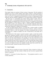
from 70 to 81 months. The results of the Weibull estimation are in Table 20.1.
In interpreting the estimates, we use equation (20.17). For small
^
bb
j

, we can multi-
ply the coe‰cient by 100 to obtain the semielasticity of the haz ard with respect to x
j
.
(No covariates appear in logarithmic form, so there are no elasticities among the
^
bb
j
.)
For example, if tserved increases by one month, the hazard shifts up by about 1.4
percent, and the e¤ect is statistically significant. Another year of education reduces
the hazard by about 2.3 percent, but the e¤ect is insignificant at even the 10 percent
level against a two-sided alternative.
The sign of the workprg coe‰cient is unexpected, at least if we expect the work
program to have positive benefits after the inmates are released from prison. (The
result is not statistically di¤erent from zero.) The reason could be that the program is
ine¤ective or that there is self-selection into the program.
For large
^
bb
j
, we should exponentiate and subtract unity to obtain the proportion-
ate change. For example, at any point in time, the hazard is about 100½expð:477 ÞÀ1
¼ 61:1 percent greater for someone with an alcohol problem than for someone
without.
Duration Analysis 697
The estimate of a is .806, and the standard error of
^
aa leads to a strong rejection of
H

0
: a ¼ 1 against H
0
: a < 1. Therefore, there is evidence of negative duration de-
pendence, conditional on the covariates. This means that, for a particular ex-convict,
the instantaneous rate of being arrested decreases with the length of time out of prison.
When the Weibull model is estimated without the covariates,
^
aa ¼ :770 (se ¼ :031),
which shows slightly more negative duration dependence. This is a typical finding in
applications of Weibull duration models: estimated a without covariate tends to be
less than the estimate with covariates. Lancaster (1990, Section 10.2) contains a the-
oretical discussion based on unobserved heterogeneity.
When we are primarily interested in the e¤ects of covariates on the expected
duration (rather than on the hazard), we can apply a censored Tobit analysis to the
Table 20.1
Weibull Estimation of Criminal Recidivism
Explanatory
Variable
Coe‰cient
(Standard Error)
workprg .091
(.091)
priors .089
(.013)
tserved .014
(.002)
felon À.299
(.106)
alcohol .447

(.106)
drugs .281
(.098)
black .454
(.088)
married À.152
(.109)
educ À.023
(.019)
age À.0037
(.0005)
constant À3.402
(0.301)
Observations 1,445
Log likelihood À1,633.03
^
aa .806
(.031)
Chapter 20698
log of the duration. A Tobit analysis assumes that, for each random draw i,logðt
Ã
i
Þ
given x
i
has a Normalðx
i
d; s
2
Þ distribution, which implies that t

Ã
i
given x
i
has a log-
normal distribution. (The first element of x
i
is unity.) The hazard function for a log-
normal distribution, conditional on x,islðt; xÞ¼h½ðlog t ÀxdÞ=s=st, where hðzÞ1
fðzÞ=½1 À FðzÞ, fðÁÞ is the standard normal probability density function (pdf ), and
FðÁÞ is the standard normal cdf. The lognormal hazard function is not monotonic
and does not have the proportional hazard form. Nevertheless, the estimates of the d
j
are easy to interpret because the model is equivalent to
logðt
Ã
i
Þ¼x
i
d þe
i
ð20:26Þ
where e
i
is independent of x
i
and normally distributed. Therefore, the d
j
are
semielasticities—or elasticities if the covariates are in logarithmic form—of the

covariates on th e expected duration.
The Weibull model can also be represented in regression form. When t
Ã
i
given x
i
has density (20.25), expðx
i
bÞðt
Ã
i
Þ
a
is independent of x
i
and has a unit exponential
distribution. Therefore, its natural log has a type I extreme value distribution; there-
fore, we can write a logðt
Ã
i
Þ¼Àx
i
b þ u
i
, where u
i
is independent of x
i
and has density
gðuÞ¼expðuÞ expfexpðÀuÞg. The mean of u

i
is not zero, but, because u
i
is indepen-
dent of x
i
, we can write logðt
Ã
i
Þ exactly as in equation (20.26), where the slope coef-
ficents are given by d
j
¼Àb
j
=a, and the intercept is more complicated. Now, e
i
does
not have a normal distribution, but it is independent of x
i
with zero mean. Censoring
can be handled by maximum likelihood estimation. The estimated coe‰cients can be
compared with the censored Tobit estimates described previously to see if the esti-
mates are sensitive to the distributional assumption.
In Example 20.5, we can obtain the Weibull estimates of the d
j
as
^
dd
j
¼À

^
bb
j
=
^
aa. (Some
econometrics packages, such as Stata, allow direct estimation of the d
j
and provide
standard errors.) For example,
^
dd
drugs
¼À:281=:806 A À:349. When the lognormal
model is used, the coe‰cient on drugs is somewhat smaller in magnitude, about
À.298. As another example,
^
dd
age
¼ :0046 in the Weibull estimation and
^
dd
age
¼ :0039
in the lognormal estimation. In both cases, the estimates have t statistics over six. For
obtaining estimates on th e expected duration, the Weibull and lognormal models give
similar results. [Interestingly, the lognormal model fits the data notably better, with
log likelihood ¼À1,597.06. This result is consistent with the findings of Chung,
Schmidt, and Witte (1991).]
Sometimes we begin by specifying a parametric model for the hazard conditional

on x and then use the formulas from Section 20.2 to obtain the cdf and density. This
approach is easiest when the hazard leads to a tractable duration distribution, but
there is no reason the hazard function must be of the proportional hazard form.
Duration Analysis 699
Example 20.6 (Log-Logistic Hazard with Covariates): A log-logistic hazard func-
tion with covariates is
lðt; xÞ¼expðxbÞat
aÀ1
=½1 þexpðxbÞt
a
ð20:27Þ
where x
1
1 1. From equation (20.14) with g ¼ expðxbÞ, the cdf is
Fðt jx; yÞ¼1 À½1 þexpðxbÞt
a

À1
; t b 0 ð20:28Þ
The distribution of logðt
Ã
i
Þ given x
i
is logistic with mean Àa
À1
logfexpðxbÞg ¼
Àa
À1
xb and variance p

2
=ð3a
2
Þ. Therefore, logðt
Ã
i
Þ can be written as in equation
(20.26) where e
i
has a zero mean logistic distribution and is independent of x
i
and
d ¼Àa
À1
b. This is another example where the e¤ects of the covariates on the mean
duration can be obtained by an OLS regressi on when there is no censoring. With
censoring, the distribution of e
i
must be accounted for using the log likelihood in
expression (20.24).
20.3.3 Stock Sampling
Flow data with right censoring are common, but other sampling schemes are also
used. With stock sampling we randomly sample from individuals that are in the initial
state at a given point in time. The population is again individuals who enter the ini-
tial state during a specified interval, ½0; b. However, rather than observe a random
sample of people flowing into the initial state, we can only obtain a random sample
of individuals that are in the initial state at time b. In addition to the possib ility of
right censoring, we may also face the problem of left censoring, which occurs when
some or all of the starting times, a
i

, are not observed. For now, we assume that (1) we
observe the starting times a
i
for all individuals we sample at time b and (2) we can
follow sampled individuals for a certain length of time after we observe them at time
b. We also allow for right censoring.
In the unemployment duration example, where the population comprises workers
who became unemployed at some point during 1998, stock sampling would occur if
we randomly sampled from workers who were unemployed during the last week of
1998. This ki nd of sampling causes a clear sample selection problem: we necessarily
exclude from our sample any individual whose unemployment spell ended before the
last week of 1998. Because these spells were necess arily shorter than a year, we can-
not just assume that the missing observations are randomly missing.
The sample selection problem caused by stock sampling is essentially the same
situation we faced in Section 17.3, where we covered the truncated regression model.
Therefore, we will call this the left truncation problem. Kiefer (1988) calls it length-
biased sampling.
Chapter 20700
Under the assumptions that we observe the a
i
and can observe some spells past
the sampling date b, left truncation is fairly easy to deal with. With the exception of
replacing flow sampling with stock sampling, we make the same assump tions as in
Section 20.3.2.
To account for the truncated sampling, we must modify the density in equation
(20.23) to reflect the fact that part of the population is systematically omitted from
the sample. Let ða
i
; c
i

; x
i
; t
i
Þ denote a random draw from the population of all spells
starting in ½0; b. We observe this vector if and only if the person is still in the initial
state at time b, that is, if and only if a
i
þ t
Ã
i
b b or t
Ã
i
b b Àa
i
, where t
Ã
i
is the true
duration. But, under the conditional independence assumption (20.22),
Pðt
Ã
i
b b Àa
i
ja
i
; c
i

; x
i
Þ¼1 ÀFðb À a
i
jx
i
; yÞð20:29Þ
where F ðÁjx
i
; yÞ is the cdf of t
Ã
i
given x
i
, as before. The correct conditional density
function is obtained by dividing equation (20.23) by equation (20.29). In Problem
20.5 you are asked to adapt the arguments in Section 17.3 to also allow for right
censoring. The log-likelihood function can be written as
X
N
i¼1
fd
i
log½ f ðt
i
jx
i
; yÞþð1 À d
i
Þ log½1 ÀF ðt

i
jx
i
; yÞÀlog½1 À Fðb Àa
i
jx
i
; yÞg
ð20:30Þ
where, again, t
i
¼ c
i
when d
i
¼ 0. Unlike in the case of flow sampling, with stock
sampling both the starting dates, a
i
, and the length of the sampling interval, b, appear
in the conditional likelihood function. Their presence makes it clear that specifying
the interval ½0; b is important for analyzing stock data. [Lancaster (1990, p. 183) es-
sentially derives equation (20.30) under a slightly di¤erent sampling scheme; see also
Lancaster (1979).]
Equation (20.30) has an interesting implication. If observation i is right censored at
calendar date b—that is, if we do not follow the spell after the initial data collection—
then the censoring time is c
i
¼ b À a
i
. Because d

i
¼ 0 for censored observations, the log
likelihood for such an observation is log½1 À Fðc
i
jx
i
; yÞ Àlog½1 À Fðb Àa
i
jx
i
; yÞ ¼
0. In other words, observations that are right censored at the data collection time
provide no information for estimating y, at least when we use equation (20.30).
Consequently, the log likel ihood in equation (20.30) does not identif y y if all units are
right censored at the interview date: equation (20.30) is identically zero. The intuition
for why equation (20.30) fails in this case is fairly clear: our data consist only of
ða
i
; x
i
Þ, and equation (20.30) is a log likelihood that is conditional on ða
i
; x
i
Þ. E¤ec-
tively, there is no random response variable.
Duration Analysis 701
Even when we censor all observ ed durations at the interview date, we can still es-
timate y, provided—at least in a parametric context—we specify a model for the
conditional distribution of the starting times, Dða

i
jx
i
Þ. (This is essentially the prob-
lem analyzed by Nickell, 1979.) We are still assuming that we observe the a
i
. So, for
example, we randomly sample from the pool of people unemployed in the last week
of 1998 and find out when their unemployment spells began (along with covariates).
We do not follow any spells past the interview date. (As an aside, if we sample un-
employed people during the last week of 1998, we are likely to obtain some obser-
vations where spells began before 1998. For the population we have specified, these
people would simply be discarded. If we want to include people whose spells began
prior to 1998, we need to redefine the interval. For example, if durations are mea-
sured in weeks and if we want to consider durations beginning in the five-year period
prior to the end of 1998, then b ¼ 260.)
For concreteness, we assume that Dða
i
jx
i
Þ is continuous on ½0; b with density
kðÁjx
i
; hÞ. Let s
i
denote a sample selection indicator, which is unity if we observe
random draw i, that is, if t
Ã
i
b b Àa

i
. Estimation of y (and h) can proceed by apply-
ing CMLE to the density of a
i
conditional on x
i
and s
i
¼ 1. [Note that this is the only
density we can hope to estimate, as our sample only consists of observations ða
i
; x
i
Þ
when s
i
¼ 1.] This density is informative for y even if h is not functionally related to y
(as would typically be assumed) because there are some durations that started and
ended in ½0; b; we simply do not observe them. Knowing something about the start-
ing time distribution gives us information about the duration distribution. (In the
context of flow sampling, when h is not functionally related to y, the density of a
i
given x
i
is uninformative for estimating y; in other words, a
i
is ancillary for y .)
In Problem 20.6 you are asked to show that the density of a
i
conditional on

observing ða
i
; x
i
Þ is
pða jx
i
; s
i
¼ 1Þ¼kða jx
i
; hÞ½1 ÀFðb À a jx
i
; yÞ=Pðs
i
¼ 1 jx
i
; y; hÞð20:31Þ
0 < a < b, where
Pðs
i
¼ 1 jx
i
; y; hÞ¼
ð
b
0
½1 ÀFðb À u jx
i
; yÞkðu jx

i
; hÞdu ð20:32Þ
[Lancaster (1990, Section 8.3.3) essentially obtains the right-hand side of equation
(20.31) but uses the notion of backward recurrence time. The argument in Problem
20.6 is more straightforward because it is based on a standard truncation argument.]
Once we have specified the duration cdf, F, and the starting time density, k, we can
use conditional MLE to estimate y and h: the log likelihood for observation i is just
the log of equation (20.31), evaluated at a
i
. If we assume that a
i
is independent of
Chapter 20702
x
i
and has a uniform distribution on ½0; b, the estimation simplifies somew hat; see
Problem 20.6. Allowing for a discontinuous starting time density kðÁjx
i
; hÞ does not
materially a¤ect equation (20.31). For example, if the interval [0,1] represents one
year, we might want to allow di¤erent entry rates over the di¤erent seasons. This
would correspond to a uniform distribution over each subinterval that we choose.
We now turn to the problem of left censoring, which arises with stock sampling
when we do not actually know when any spell began. In other words, the a
i
are not
observed, and therefore neither are the true durations, t
Ã
i
. However, we assume that

we can follow spells after the interview date. Without right censoring, this assump-
tion means we can observe the time in the current spell since the interview date, say,
r
i
, which we can write as r
i
¼ t
Ã
i
þ a
i
À b. We still have a left truncation problem
because we only observe r
i
when t
Ã
i
> b À a
i
, that is, when r
i
> 0. The general
approach is the same as with the earlier problems: we obtain the density of the vari-
able that we can at least partially observe, r
i
in this case, conditional on observing
r
i
. Problem 20.8 asks you to fill in the details, accounting also for possible right
censoring.

We can easily combine stock sampling and flow sampling. For example, in the case
that we observe the starting times, a
i
, suppose that, at time m < b, we sample a stock
of individuals already in the initial state. In addition to following spells of individuals
already in the initial state, suppose we can randomly sample individuals flowing into
the initial state between times m and b. Then we follow all the individuals appearing
in the sample, at least until right censor ing. For starting dates after m ða
i
b mÞ, there
is no truncation, and so the log likelihood for these observations is just as in equation
(20.24). For a
i
< m, the log likelihood is identical to equation (20.30) except that m
replaces b. Other combinations are easy to infer from the preceding results.
20.3.4 Unobserved Heterogeneity
One way to obtain more general duration models is to introduce unobserved hetero-
geneity into fairly simple duration models. In addition, we sometimes want to test for
duration dependence conditional on observ ed covariates and unobserved heteroge-
neity. The key assumptions used in most models that incorporate unobserved heter-
ogeneity are that (1) the heterogeneity is independent of the observed covariates, as
well as starting times and censoring times; (2) the heterogeneity has a distribution
known up to a finite number of parameters; and (3) the heterogeneity enters the
hazard function multiplicatively. We will make these assumptions. In the context of
single-spell flow data, it is di‰cult to relax any of these assumptions. (In the special
case of a lognormal duration distribution, we can relax assumption 1 by using Tobit
methods with endogenous explanatory variables; see Section 16.6.2.)
Duration Analysis 703
Before we cover the general case, it is useful to cover an example due to Lancaster
(1979). For a random draw i from the population, a Weibull hazard function condi-

tional on observed covariates x
i
and unobserved heterogeneity v
i
is
lðt; x
i
; v
i
Þ¼v
i
expðx
i
bÞat
aÀ1
ð20:33Þ
where x
i1
1 1 and v
i
> 0. [Lancaster (1990) calls equation (20.33) a conditional haz-
ard, because it conditions on the unobserved heterogeneity v
i
. Technically, almost all
hazards in econometrics are conditional because we almost always condition on
observed covariates.] Notice how v
i
enters equation (20.33) multiplicatively. To
identify the parameters a and b we need a normalization on the distribution of v
i

;we
use the most common, Eðv
i
Þ¼1. This implies that, for a given vector x, the average
hazard is expðxbÞat
aÀ1
. An interesting hypothesis is H
0
: a ¼ 1, which means that,
conditional on x
i
and v
i
, there is no duration dependence.
In the general case where the cdf of t
Ã
i
given ðx
i
; v
i
Þ is Fðt jx
i
; v
i
; yÞ, we can obtain
the distribution of t
Ã
i
given x

i
by integrating out the unobserved e¤ect. Because v
i
and
x
i
are independent, the cdf of t
Ã
i
given x
i
is
Gðt jx
i
; y; rÞ¼
ð
y
0
Fðt jx
i
; v; yÞhðv; rÞdv ð20:34Þ
where, for concreteness, the density of v
i
, hðÁ; rÞ, is assumed to be continuous and
depends on the unknown parameters r. From equation (20.34) the density of t
Ã
i
given
x
i

, gðt jx
i
; y; rÞ, is easily obtained. We can now use the methods of Sections 20.3.2
and 20.3.3. For flow data, the log-likelihood function is as in equation (20.24), but
with Gðt jx
i
; y; rÞ replacing F ð t jx
i
; yÞ and gðt jx
i
; y; rÞ replacing f ðt jx
i
; yÞ.We
should assume that Dðt
Ã
i
jx
i
; v
i
; a
i
; c
i
Þ¼Dðt
Ã
i
jx
i
; v

i
Þ and D ðv
i
jx
i
; a
i
; c
i
Þ¼Dðv
i
Þ;
these assumptions ensure that the key condition (20.22) holds. The methods for stock
sampling described in Section 20.3.3 also apply to the integrated cdf and density.
If we assume gamma-distributed heterogeneity—that is, v
i
@ Gammaðd; dÞ, so that
Eðv
i
Þ¼1 and Varðv
i
Þ¼1=d—we can find the distribution of t
Ã
i
given x
i
for a broad
class of hazard functions with multiplicative heterogeneity. Suppose that the hazard
function is lðt; x
i

; v
i
Þ¼v
i
kðt; x
i
Þ, where kðt; xÞ > 0 (and need not have the propor-
tional hazard form). For simplicity, we suppress the dependence of kðÁ; ÁÞ on un-
known parameters. From equation (20.7), the cdf of t
Ã
i
given ðx
i
; v
i
Þ is
Fðt jx
i
; v
i
Þ¼1 Àexp Àv
i
ð
t
0
kðs; x
i
Þds
!
1 1 Àexp½Àv

i
xðt; x
i
Þ ð20:35Þ
where xðt; x
i
Þ1
Ð
t
0
kðs; x
i
Þds. We can obtain the cdf of t
Ã
i
given x
i
by using equation
(20.34). The density of v
i
is hðvÞ¼d
d
v
dÀ1
expðÀdvÞ=GðdÞ, where Varðv
i
Þ¼1=d and
Chapter 20704
GðÁÞ is the gamma function. Let x
i

1 xðt; x
i
Þ for given t. Then
ð
y
0
expðÀx
i
vÞd
d
v
dÀ1
expðÀdvÞ=GðdÞdv
¼½d = ðd þx
i
Þ
d
ð
y
0
ðd þx
i
Þ
d
v
dÀ1
exp½Àðd þx
i
Þv=GðdÞdv
¼½d = ðd þx

i
Þ
d
¼ð1 þ x
i
=dÞ
Àd
where the second-to-last equality follows because the integrand is the Gamma ðd;
d þx
i
Þ density and must integrate to unity. Now we use equation (20.34):
Gðt jx
i
Þ¼1 À½1 þxðt; x
i
Þ=d
Àd
ð20:36Þ
Taking the derivative of equation (20.36) with respect to t, using the fact that kðt; x
i
Þ
is the derivative of xðt; x
i
Þ, yields the density of t
Ã
i
given x
i
as
gðt jx

i
Þ¼kðt; x
i
Þ½1 þxðt; x
i
Þ=d
ÀðdÀ1Þ
ð20:37Þ
The function kðt; xÞ depends on parameters y, and so gðt jxÞ should be gðt jx; y; dÞ.
With censored data the vector y can be estimated along with d by using the log-
likelihood function in equation (20.24) (again, with G replacing F ).
With the Weibull hazard in equation (20.33), xðt; xÞ¼expðxb Þt
a
, which leads to a
very tractable analysis when plugged into equations (20.36) and (20.37); the resulting
duration distribution is called the Burr distribution. In the log-logistic case with
kðt; xÞ¼expðxb Þat
aÀ1
½1 þexpðxbÞt
a

À1
, xðt; xÞ¼log½1 þexpðxbÞt
a
. These equa-
tions can be plugged into the preceding formulas for a maximum likelihood analysis.
Before we end this section, we should recall why we might want to explicitly in-
troduce unobserved heterogeneity when the heterogeneity is assumed to be indepen-
dent of the observed covariates. The strongest case is seen when we a re interested in
testing for duration dependence conditional on observed covariates and unobserved

heterogeneity, where the unobserved heterogeneity enters the hazard multiplicatively.
As carefully exposited by Lancaster (1990, Section 10.2), igno ring multiplicative
heterogeneity in the Weibull model results in asymptotically underestimating a.
Therefore, we could very well conclude that there is negative duration dependence
conditional on x, whereas there is no duration dependence ða ¼ 1Þ conditional on x
and v.
In a general sense, it is somewhat heroic to think we can distinguish between dura-
tion dependence and unobserved heterogeneity when we observe only a single cycle
for each agent. The problem is simple to describe: because we can only estimate the
distribution of T given x, we cannot uncover the distribution of T given ðx; vÞ unless
Duration Analysis 705
we make extra assumptions, a point Lancaster (1990, Section 10.1) illustrates with an
example. Therefore, we cannot tell whether the hazar d describing T given ðx; vÞ
exhibits duration dependence. But, when the hazard has the proportional hazard
form lðt; x; vÞ¼vkðxÞl
0
ðtÞ, it is possible to identify the function kðÁÞ and the baseline
hazard l
0
ðÁÞ quite generally (along with the distribution of v). See Lancaster (1990,
Section 7.3) for a presentation of the results of Elbers and Ridd er (1982). Recently,
Horowitz (1999) has demonstrated how to nonparametrically estimate the baseline
hazard and the distribution of the unobserved heterogeneity under fairly weak
assumptions.
When interest centers on how the observed covariate s a¤ect the mean duration,
explicitly modeling unobserved heterogeneity is less compelling. Adding unobserved
heterogeneity to equation (20.26) does not change the mean e¤ects; it merely changes
the error distribution. Without censoring, we would probably estim ate b in equation
(20.26) by OLS (rather than MLE) so that the estimators would be robust to dis-
tributional misspecification. With censoring, to perform maximum likelihood, we

must know the distribution of t
Ã
i
given x
i
, and this depends on the distribution of v
i
when we explicitly introduce unobserved heterogeneity. But introducing unobserved
heterogeneity is indistinguishable from simply allowing a more flexible duration dis-
tribution.
20.4 Analysis of Grouped Duration Data
Continuously distributed durations are, strictly spe aking, rare in social science appli-
cations. Even if an underlying duration is properly viewed as being continuous, mea-
surements are necessarily discrete. When the measurements are fairly precise, it is
sensible to treat the durations as continuous random variables. But when the mea-
surements are coarse—such as monthly, or perhaps even weekly—it can be impor-
tant to account for the discreteness in the estimation.
Grouped duration data arise when each duration is only known to fall into a certain
time interval, such as a week, a month, or even a year. For example, unemployment
durations are often measured to the nearest week. In Example 20.2 the time until next
arrest is measured to the nearest month. Even with grouped data we can generally
estimate the parameters of the duration distribution.
The approach we take here to analyzing grouped data summarizes the information
on staying in the initial state or exiting in each time interval in a sequence of binary
outcomes. (Kiefer, 1988; Han and Hausman, 1990; Meyer, 1990; Lancaster, 1990;
McCall, 1994; and Sueyoshi, 1995, all take this approach.) In e¤ect, we have a panel
data set where each cross section observation is a vector of binary responses, along
Chapter 20706
with covariates. In addition to allowing us to treat grouped durations, the panel data
approach has at least two additional advantages. First, in a proportional hazard

specification, it leads to easy methods for estimating flexible hazard functions. Sec-
ond, bec ause of the sequential nature of the data, time-varying covariates are easily
introduced.
We assume flow sampling so that we do not have to address the sample selection
problem that arises with stock sampling. We divide the time line into M þ 1 inter-
vals, ½0; a
1
Þ; ½a
1
; a
2
Þ; ; ½a
MÀ1
; a
M
Þ; ½a
M
; yÞ, where the a
m
are known constants. For
example, we might have a
1
¼ 1; a
2
¼ 2; a
3
¼ 3, and so on, but unequally spaced
intervals are allowed. The last interval, ½a
M
; yÞ, is chosen so that any duration fall-

ing into it is censored at a
M
: no observed durations are greater than a
M
. For a ran-
dom draw from the population, let c
m
be a binary censoring indicator equal to unity
if the duration is censored in interval m, and zero otherwise. Notice that c
m
¼ 1
implies c
mþ1
¼ 1: if the duration was censored in interval m, it is still censored in in-
terval m þ1. Because durations lasting into the last interval are censored, c
Mþ1
1 1.
Similarly, y
m
is a bin ary indicator equal to unity if the duration ends in the mth in-
terval and zero otherwise. Thus, y
mþ1
¼ 1ify
m
¼ 1. If the duration is censored in
interval m ðc
m
¼ 1Þ, we set y
m
1 1 by convention.

As in Section 20.3, we allow individuals to enter the initial state at di¤erent calen-
dar times. In order to keep the notation simple, we do not explicitly show the con-
ditioning on these starting times, as the starting times play no role under flow
sampling when we assume that, condit ional on the covariates, the starting times are
independent of the duration and any unobserved heterogeneity. If necessary, starting-
time dummies can be included in the covariates.
For each person i, we observe ðy
i1
; c
i1
Þ; ; ðy
iM
; c
iM
Þ, which is a balanced panel
data set. To avoid confusion with our notation for a duratio n (T for the random
variable, t fo r a particular outcome on T ), we use m to index the time intervals. The
string of binary indicators fo r any individual is not unrestricted: we must observe a
string of zeros followed by a string of ones. The important information is the interval
in which y
im
becomes unity for the first time, and whether that represents a true exit
from the initial state or censoring.
20.4.1 Time-Invariant Covariates
With time-invariant covariates, each random draw from the population consists of
information on fðy
1
; c
1
Þ; ; ðy

M
; c
M
Þ; xg. We assume that a parametric hazard
function is specified as lðt; x; yÞ, where y is the vector of unknown parameters. Let T
denote the time until exit from the initial state. While we do not fully observe T,
either we know which interval it falls into, or we know whether it was censored in a
Duration Analysis 707
particular interval. This knowledge is enough to obtain the probability that y
m
takes
on the value unity given ðy
mÀ1
; ; y
1
Þ, ðc
m
; ; c
1
Þ, and x. In fact, by definition this
probability depends only on y
mÀ1
, c
m
, and x, and only two combinations yield
probabilities that are not identically zero or one. These probabilities are
Pðy
m
¼ 0 j y
mÀ1

¼ 0; x; c
m
¼ 0Þð20:38Þ
Pðy
m
¼ 1 j y
mÀ1
¼ 0; x; c
m
¼ 0Þ; m ¼ 1; ; M ð20:39Þ
(We define y
0
1 0 so that these equations hol d for all m b 1.) To compute these
probabilities in terms of the hazard for T, we assume that the duration is condition-
ally independent of censoring:
T is independent of c
1
; ; c
M
, given x ð20:40Þ
This assumption allows the censoring to depend on x but rules out censoring that
depends on unobservables, after conditioning on x. Condition (20.40) holds for fixed
censoring or completely randomized censoring. (It may not hold if censoring is due to
nonrandom attrition.) Under assumption (20.40) we have, from equation (20.9),
Pðy
m
¼ 1 j y
mÀ1
¼ 0; x; c
m

¼ 0Þ¼Pða
mÀ1
a T < a
m
jT b a
mÀ1
; xÞ
¼ 1 À exp À
ð
a
m
a
mÀ1
lðs; x; yÞds
!
1 1 Àa
m
ðx; yÞ
ð20:41Þ
for m ¼ 1; 2; ; M, where
a
m
ðx; yÞ1 exp À
ð
a
m
a
mÀ1
lðs; x; yÞds
!

ð20:42Þ
Therefore,
Pðy
m
¼ 0 j y
mÀ1
¼ 0; x; c
m
¼ 0Þ¼a
m
ðx; yÞð20:43Þ
We can use these probabilities to construct the likelihood function. If, for observation
i, uncensored exit occurs in interval m
i
, the likelihood is
Y
m
i
À1
h¼1
a
h
ðx
i
; yÞ
"#
½1 Àa
m
i
ðx

i
; yÞ ð20:44Þ
The first term represents the probability of remaining in the initial state for the first
m
i
À 1 intervals, and the second term is the (conditional) probability that T falls into
interval m
i
. [Because an uncensored duration must have m
i
a M, expression (20.44)
Chapter 20708
at most depends on a
1
ðx
i
; yÞ; ; a
M
ðx
i
; yÞ.] If the duration is censored in interval m
i
,
we know only that exit did not occur in the first m
i
À 1 intervals, and the likelihood
consists of onl y the first term in expression (20.44).
If d
i
is a censoring indicator equal to one if duration i is uncensored, the log like-

lihood for observation i can be written as
X
m
i
À1
h¼1
log½a
h
ðx
i
; yÞ þd
i
log½1 Àa
m
i
ðx
i
; yÞ ð20:45Þ
The log likelihood for the entire sample is obtained by summing expression (20.45)
across all i ¼ 1; ; N. Under the assumptions made, this log likelihood represents
the density of ðy
1
; ; y
M
Þ given ðc
1
; ; c
M
Þ and x, and so the conditional maxi-
mum likelihood theory covered in Chapter 13 applies directly. The various ways of

estimating asymptotic variances and computing test statistics are available.
To implement conditional MLE, we must specify a hazard function. One hazard
function that has become popular because of its flexibility is a piecewise-constant
proportional hazard: for m ¼ 1; ; M,
lðt; x; yÞ¼kðx; bÞl
m
; a
mÀ1
a t < a
m
ð20:46Þ
where kðx; bÞ > 0 [and typically kðx; bÞ¼expðxbÞ]. This specification allows the
hazard to be di¤erent (albeit constant) ove r each time interval. The parameters to be
estimated are b and l, where the latter is the vector of l
m
, m ¼ 1; ; M. {Because
durations in ½a
M
; yÞ are censored at a
M
, we cannot estimate the hazard over the
interval ½a
M
; yÞ.} As an example, if we have unemployment duration measured in
weeks, the hazard can be di¤erent in each week. If the durations are sparse, we might
assume a di¤erent hazard rate for every two or three weeks (this assumption places
restrictions on the l
m
). With the piecewise-constant hazard and kðx; bÞ¼expðxb Þ,
for m ¼ 1; ; M, we have

a
m
ðx; yÞ1 exp½ÀexpðxbÞl
m
ða
m
À a
mÀ1
Þ ð20:47Þ
Remember, the a
m
are known constants (often a
m
¼ m) and not parameters to
be estimated. Usually the l
m
are unrestricted, in which case x does not contain an
intercept.
The piecewise-constant hazard implies that the duration distribution is discontin-
uous at the endpoints, whereas in our discussion in Section 20.2, we assumed that the
duration had a continuous distribution. A piecewise-continuous distribution causes
no real problems, and the log likelihood is exactly as specified previously. Alter-
natively, as in Han and Hausman (1990) and Meyer (1990), we can assume that T
Duration Analysis 709