From Individuals to Ecosystems 4th Edition - Chapter 1 pptx

••
Introduction
We have chosen to start this book with chapters about organ-
isms, then to consider the ways in which they interact with each
other, and lastly to consider the properties of the communities
that they form. One could call this a ‘constructive’ approach. We
could though, quite sensibly, have treated the subject the other
way round – starting with a discussion of the complex com-
munities of both natural and manmade habitats, proceeding to
deconstruct them at ever finer scales, and ending with chapters
on the characteristics of the individual organisms – a more
analytical approach. Neither is ‘correct’. Our approach avoids
having to describe community patterns before discussing the
populations that comprise them. But when we start with individual
organisms, we have to accept that many of the environmental
forces acting on them, especially the species with which they
coexist, will only be dealt with fully later in the book.
This first section covers individual organisms and populations
composed of just a single species. We consider initially the sorts
of correspondences that we can detect between organisms and
the environments in which they live. It would be facile to start
with the view that every organism is in some way ideally fitted
to live where it does. Rather, we emphasize in Chapter 1 that
organisms frequently are as they are, and live where they do,
because of the constraints imposed by their evolutionary history.
All species are absent from almost everywhere, and we consider
next, in Chapter 2, the ways in which environmental conditions
vary from place to place and from time to time, and how these
put limits on the distribution of particular species. Then, in
Chapter 3, we look at the resources that different types of
organisms consume, and the nature of their interactions with

these resources.
The particular species present in a community, and their
abundance, give that community much of its ecological interest.
Abundance and distribution (variation in abundance from place
to place) are determined by the balance between birth, death, immi-
gration and emigration. In Chapter 4 we consider some of the
variety in the schedules of birth and death, how these may be
quantified, and the resultant patterns in ‘life histories’: lifetime
profiles of growth, differentiation, storage and reproduction. In
Chapter 5 we examine perhaps the most pervasive interaction
acting within single-species populations: intraspecific competition
for shared resources in short supply. In Chapter 6 we turn to move-
ment: immigration and emigration. Every species of plant and
animal has a characteristic ability to disperse. This determines the
rate at which individuals escape from environments that are or
become unfavorable, and the rate at which they discover sites
that are ripe for colonization and exploitation. The abundance
or rarity of a species may be determined by its ability to disperse
(or migrate) to unoccupied patches, islands or continents. Finally
in this section, in Chapter 7, we consider the application of the
principles that have been discussed in the preceding chapters, includ-
ing niche theory, life history theory, patterns of movement, and
the dynamics of small populations, paying particular attention
to restoration after environmental damage, biosecurity (resisting
the invasion of alien species) and species conservation.
Part 1
Organisms
EIPC01 10/24/05 1:42 PM Page 1
••
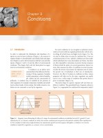
1.1 Introduction: natural selection and

adaptation
From our definition of ecology in the Preface, and even from a
layman’s understanding of the term, it is clear that at the heart
of ecology lies the relationship between organisms and their
environments. In this opening chapter we explain how, funda-
mentally, this is an evolutionary relationship. The great Russian–
American biologist Theodosius Dobzhansky famously said:
‘Nothing in biology makes sense, except in the light of evolution’.
This is as true of ecology as of any other aspect of biology. Thus,
we try here to explain the processes by which the properties
of different sorts of species make their life possible in particular
environments, and also to explain their failure to live in other
environments. In mapping out this evolutionary backdrop to the
subject, we will also be introducing many of the questions that
are taken up in detail in later chapters.
The phrase that, in everyday speech, is most commonly used
to describe the match between organisms and environment is:
‘organism X is adapted to’ followed by a description of where the
organism is found. Thus, we often hear that ‘fish are adapted to
live in water’, or ‘cacti are adapted to live in conditions of drought’.
In everyday speech, this may mean very little: simply that fish have
characteristics that allow them to live in water (and perhaps exclude
them from other environments) or that cacti have characteristics
that allow them to live where water is scarce. The word ‘adapted’
here says nothing about how the characteristics were acquired.
For an ecologist or evolutionary
biologist, however, ‘X is adapted to
live in Y’ means that environment Y has
provided forces of natural selection
that have affected the life of X’s ancestors and so have molded

and specialized the evolution of X. ‘Adaptation’ means that
genetic change has occurred.
Regrettably, though, the word ‘adaptation’ implies that
organisms are matched to their present environments, suggest-
ing ‘design’ or even ‘prediction’. But organisms have not been
designed for, or fitted to the present: they have been molded
(by natural selection) by past environments. Their characteristics
reflect the successes and failures of ancestors. They appear to
be apt for the environments that they live in at present only
because present environments tend to be similar to those of
the past.
The theory of evolution by natural selection is an ecological
theory. It was first elaborated by Charles Darwin (1859), though
its essence was also appreciated by a contemporary and corres-
pondent of Darwin’s, Alfred Russell
Wallace (Figure 1.1). It rests on a series
of propositions.
1 The individuals that make up a population of a species are not
identical: they vary, although sometimes only slightly, in size,
rate of development, response to temperature, and so on.
2 Some, at least, of this variation is heritable. In other words,
the characteristics of an individual are determined to some
extent by its genetic make-up. Individuals receive their
genes from their ancestors and therefore tend to share their
characteristics.
3 All populations have the potential to populate the whole earth,
and they would do so if each individual survived and each indi-
vidual produced its maximum number of descendants. But they
do not: many individuals die prior to reproduction, and most
(if not all) reproduce at a less than maximal rate.

4 Different ancestors leave different numbers of descendants. This
means much more than saying that different individuals produce
different numbers of offspring. It includes also the chances
of survival of offspring to reproductive age, the survival and
reproduction of the progeny of these offspring, the survival
and reproduction of their offspring in turn, and so on.
5 Finally, the number of descendants that an individual leaves
depends, not entirely but crucially, on the interaction between
the characteristics of the individual and its environment.
the meaning of
adaptation
evolution by natural
selection
Chapter 1
Organisms in
their Environments:
the Evolutionary Backdrop
EIPC01 10/24/05 1:42 PM Page 3
4 CHAPTER 1
In any environment, some individuals will tend to survive
and reproduce better, and leave more descendants, than others.
If, because of this, the heritable characteristics of a population
change from generation to generation, then evolution by nat-
ural selection is said to have occurred. This is the sense in which
nature may loosely be thought of as selecting. But nature does not
select in the way that plant and animal breeders select. Breeders
have a defined end in view – bigger seeds or a faster racehorse.
But nature does not actively select in this way: it simply sets the
scene within which the evolutionary play of differential survival
and reproduction is played out.

The fittest individuals in a popula-
tion are those that leave the greatest
number of descendants. In practice,
the term is often applied not to a single individual, but to a typ-
ical individual or a type. For example, we may say that in sand
dunes, yellow-shelled snails are fitter than brown-shelled snails.
Fitness, then, is a relative not an absolute term. The fittest indi-
viduals in a population are those that leave the greatest number
of descendants relative to the number of descendants left by
other individuals in the population.
When we marvel at the diversity
of complex specializations, there is a
temptation to regard each case as an
example of evolved perfection. But this would be wrong. The
evolutionary process works on the genetic variation that is avail-
able. It follows that natural selection is unlikely to lead to the
evolution of perfect, ‘maximally fit’ individuals. Rather, organisms
••••
Figure 1.1 (a) Charles Darwin, 1849 (lithograph by Thomas H.
Maguire; courtesy of The Royal Institution, London,
UK/Bridgeman Art Library). (b) Alfred Russell Wallace, 1862
(courtesy of the Natural History Museum, London).
fitness: it’s all relative
evolved perfection?
no
(a) (b)
EIPC01 10/24/05 1:42 PM Page 4
THE EVOLUTIONARY BACKDROP 5
come to match their environments by being ‘the fittest available’
or ‘the fittest yet’: they are not ‘the best imaginable’. Part of the

lack of fit arises because the present properties of an organism
have not all originated in an environment similar in every
respect to the one in which it now lives. Over the course of its
evolutionary history (its phylogeny), an organism’s remote an-
cestors may have evolved a set of characteristics – evolutionary
‘baggage’ – that subsequently constrain future evolution. For
many millions of years, the evolution of vertebrates has
been limited to what can be achieved by organisms with a ver-
tebral column. Moreover, much of what we now see as precise
matches between an organism and its environment may equally
be seen as constraints: koala bears live successfully on Eucalyptus
foliage, but, from another perspective, koala bears cannot live
without Eucalyptus foliage.
1.2 Specialization within species
The natural world is not composed of a continuum of types of
organism each grading into the next: we recognize boundaries
between one type of organism and another. Nevertheless, within
what we recognize as species (defined below), there is often con-
siderable variation, and some of this is heritable. It is on such
intraspecific variation, after all, that plant and animal breeders (and
natural selection) work.
Since the environments experienced by a species in different
parts of its range are themselves different (to at least some
extent), we might expect natural selection to have favored dif-
ferent variants of the species at different sites. The word ‘ecotype’
was first coined for plant populations (Turesson, 1922a, 1922b)
to describe genetically determined differences between popula-
tions within a species that reflect local matches between the
organisms and their environments. But evolution forces the
characteristics of populations to diverge from each other only if:

(i) there is sufficient heritable variation on which selection can
act; and (ii) the forces favoring divergence are strong enough to
counteract the mixing and hybridization of individuals from dif-
ferent sites. Two populations will not diverge completely if their
members (or, in the case of plants, their pollen) are continually
migrating between them and mixing their genes.
Local, specialized populations become differentiated most
conspicuously amongst organisms that are immobile for most of
their lives. Motile organisms have a large measure of control over
the environment in which they live; they can recoil or retreat from
a lethal or unfavorable environment and actively seek another.
Sessile, immobile organisms have no such freedom. They must
live, or die, in the conditions where they settle. Populations
of sessile organisms are therefore exposed to forces of natural
selection in a peculiarly intense form.
This contrast is highlighted on the seashore, where the inter-
tidal environment continually oscillates between the terrestrial and
the aquatic. The fixed algae, sponges, mussels and barnacles all
meet and tolerate life at the two extremes. But the mobile
shrimps, crabs and fish track their aquatic habitat as it moves; whilst
the shore-feeding birds track their terrestrial habitat. The mobil-
ity of such organisms enables them to match their environments
to themselves. The immobile organism must match itself to its
environment.
1.2.1 Geographic variation within species: ecotypes
The sapphire rockcress, Arabis fecunda, is a rare perennial herb
restricted to calcareous soil outcrops in western Montana (USA)
– so rare, in fact, that there are just 19 existing populations
separated into two groups (‘high elevation’ and ‘low elevation’)
by a distance of around 100 km. Whether there is local adapta-

tion is of practical importance for conservation: four of the low
elevation populations are under threat from spreading urban
areas and may require reintroduction from elsewhere if they are
to be sustained. Reintroduction may fail if local adaptation is too
marked. Observing plants in their own habitats and checking
for differences between them would not tell us if there was local
adaptation in the evolutionary sense. Differences may simply be
the result of immediate responses to contrasting environments
made by plants that are essentially the same. Hence, high and low
elevation plants were grown together in a ‘common garden’, elim-
inating any influence of contrasting immediate environments
(McKay et al., 2001). The low elevation sites were more prone to
drought; both the air and the soil were warmer and drier. The
low elevation plants in the common garden were indeed
significantly more drought tolerant (Figure 1.2).
On the other hand, local selection by
no means always overrides hybridization.
For example, in a study of Chamaecrista
fasciculata, an annual legume from
disturbed habitats in eastern North
America, plants were grown in a common garden that were derived
from the ‘home’ site or were transplanted from distances of
0.1, 1, 10, 100, 1000 and 2000 km (Galloway & Fenster, 2000).
The study was replicated three times: in Kansas, Maryland and
northern Illinois. Five characteristics were measured: germination,
survival, vegetative biomass, fruit production and the number
of fruit produced per seed planted. But for all characters in all
replicates there was little or no evidence for local adaptation
except at the very furthest spatial scales (e.g. Figure 1.3). There
is ‘local adaptation’ – but it’s clearly not that local.

We can also test whether organisms have evolved to become
specialized to life in their local environment in reciprocal transplant
experiments: comparing their performance when they are grown
‘at home’ (i.e. in their original habitat) with their performance
‘away’ (i.e. in the habitat of others). One such experiment (con-
cerning white clover) is described in the next section.
••••
the balance between
local adaptation and
hybridization
EIPC01 10/24/05 1:42 PM Page 5
6 CHAPTER 1
1.2.2 Genetic polymorphism
On a finer scale than ecotypes, it
may also be possible to detect levels
of variation within populations. Such
variation is known as polymorphism.
Specifically, genetic polymorphism is ‘the occurrence together
in the same habitat of two or more discontinuous forms of a species
in such proportions that the rarest of them cannot merely be
maintained by recurrent mutation or immigration’ (Ford, 1940).
Not all such variation represents a match between organism and
environment. Indeed, some of it may represent a mismatch, if,
for example, conditions in a habitat change so that one form is
being replaced by another. Such polymorphisms are called tran-
sient. As all communities are always changing, much polymor-
phism that we observe in nature may be transient, representing
••••
High
elevation

3
2
1
0
Water-use efficiency
(mols of CO
2
gained per mol of H
2
O lost × 10
–3
)
Low
elevation
High
elevation
20
15
10
0
Rosette height (mm)
Low
elevation
High
elevation
40
20
10
0
Rosette diameter (mm)

Low
elevation
P = 0.009 P = 0.0001 P = 0.001
5
30
Figure 1.2 When plants of the rare sapphire rockcress from low elevation (drought-prone) and high elevation sites were grown together
in a common garden, there was local adaptation: those from the low elevation site had significantly better water-use efficiency as well as
having both taller and broader rosettes. (From McKay et al., 2001.)
200010001001010.10
0
30
60
90
Germination (%)
Transplant distance (km)
*
*
transient
polymorphisms
Figure 1.3 Percentage germination
of local and transplanted Chamaecrista
fasciculata populations to test for local
adaptation along a transect in Kansas. Data
for 1995 and 1996 have been combined
because they do not differ significantly.
Populations that differ from the home
population at P < 0.05 are indicated by an
asterisk. Local adaptation occurs at only
the largest spatial scales. (From Galloway
& Fenster, 2000.)

EIPC01 10/24/05 1:42 PM Page 6
THE EVOLUTIONARY BACKDROP 7
the extent to which the genetic response of populations to
environmental change will always be out of step with the
environment and unable to anticipate changing circumstances
– this is illustrated in the peppered moth example below.
Many polymorphisms, however, are
actively maintained in a population by
natural selection, and there are a num-
ber of ways in which this may occur.
1 Heterozygotes may be of superior fitness, but because of the
mechanics of Mendelian genetics they continually generate less
fit homozygotes within the population. Such ‘heterosis’ is
seen in human sickle-cell anaemia where malaria is prevalent.
The malaria parasite attacks red blood cells. The sickle-cell muta-
tion gives rise to red cells that are physiologically imperfect
and misshapen. However, sickle-cell heterozygotes are fittest
because they suffer only slightly from anemia and are little
affected by malaria; but they continually generate homozygotes
that are either dangerously anemic (two sickle-cell genes) or
susceptible to malaria (no sickle-cell genes). None the less, the
superior fitness of the heterozygote maintains both types of
gene in the population (that is, a polymorphism).
2 There may be gradients of selective forces favoring one form
(morph) at one end of the gradient, and another form at the
other. This can produce polymorphic populations at inter-
mediate positions in the gradient – this, too, is illustrated
below in the peppered moth study.
3 There may be frequency-dependent selection in which each of
the morphs of a species is fittest when it is rarest (Clarke &

Partridge, 1988). This is believed to be the case when rare color
forms of prey are fit because they go unrecognized and are
therefore ignored by their predators.
4 Selective forces may operate in different directions within different
patches in the population. A striking example of this is provided
by a reciprocal transplant study of white clover (Trifolium
repens) in a field in North Wales (UK). To determine whether
the characteristics of individuals matched local features of
their environment, Turkington and Harper (1979) removed
plants from marked positions in the field and multiplied them
into clones in the common environment of a greenhouse. They
then transplanted samples from each clone into the place in
the sward of vegetation from which it had originally been taken
(as a control), and also to the places from where all the
others had been taken (a transplant). The plants were allowed
to grow for a year before they were removed, dried and
weighed. The mean weight of clover plants transplanted back
into their home sites was 0.89 g but at away sites it was only
0.52 g, a statistically highly significant difference. This provides
strong, direct evidence that clover clones in the pasture had
evolved to become specialized such that they performed best
in their local environment. But all this was going on within a
single population, which was therefore polymorphic.
In fact, the distinction between
local ecotypes and polymorphic popu-
lations is not always a clear one. This
is illustrated by another study in North
Wales, where there was a gradation in
habitats at the margin between maritime cliffs and grazed
pasture, and a common species, creeping bent grass (Agrostis

stolonifera), was present in many of the habitats. Figure 1.4 shows
a map of the site and one of the transects from which plants were
sampled. It also shows the results when plants from the sampling
points along this transect were grown in a common garden. The
••••
Figure 1.4 (a) Map of Abraham’s Bosom,
the site chosen for a study of evolution
over very short distances. The darker
colored area is grazed pasture; the lighter
areas are the cliffs falling to the sea. The
numbers indicate the sites from which the
grass Agrostis stolonifera was sampled. Note
that the whole area is only 200 m long.
(b) A vertical transect across the study area
showing the gradual change from pasture
to cliff conditions. (c) The mean length
of stolons produced in the experimental
garden from samples taken from the
transect. (From Aston & Bradshaw, 1966.)
the maintenance of
polymorphisms
no clear distinction
between local
ecotypes and a
polymorphism
1
2
3
4
5

N
0 200 m100
Irish
Sea
(a)
1
2
3
5
4
100
30
20
10
0
Elevation (m)
0
(b)
100
50
25
0
Stolon length (cm)
0
(c)
Distance (m)
EIPC01 10/24/05 1:42 PM Page 7
8 CHAPTER 1
plants spread by sending out shoots along the ground surface
(stolons), and the growth of plants was compared by measuring

the lengths of these. In the field, cliff plants formed only short
stolons, whereas those of the pasture plants were long. In the experi-
mental garden, these differences were maintained, even though
the sampling points were typically only around 30 m apart –
certainly within the range of pollen dispersal between plants. Indeed,
the gradually changing environment along the transect was
matched by a gradually changing stolon length, presumably with
a genetic basis, since it was apparent in the common garden. Thus,
even though the spatial scale was so small, the forces of selection
seem to outweigh the mixing forces of hybridization – but it is a
moot point whether we should describe this as a small-scale
series of local ecotypes or a polymorphic population maintained
by a gradient of selection.
1.2.3 Variation within a species with manmade
selection pressures
It is, perhaps, not surprising that some of the most dramatic
examples of local specialization within species (indeed of natural
selection in action) have been driven by manmade ecological forces,
especially those of environmental pollution. These can provide
rapid change under the influence of powerful selection pressures.
Industrial melanism, for example, is the phenomenon in which black
or blackish forms of species have come to dominate populations
in industrial areas. In the dark individuals, a dominant gene is typ-
ically responsible for producing an excess of the black pigment
melanin. Industrial melanism is known in most industrialized coun-
tries and more than 100 species of moth have evolved forms of
industrial melanism.
••••
f. insularia
f. carbonaria

f. typica
Figure 1.5 Sites in Britain where the
frequencies of the pale ( forma typica) and
melanic forms of Biston betularia were
recorded by Kettlewell and his colleagues.
In all more than 20,000 specimens were
examined. The principal melanic form
( forma carbonaria) was abundant near
industrial areas and where the prevailing
westerly winds carry atmospheric pollution
to the east. A further melanic form ( forma
insularia, which looks like an intermediate
form but is due to several different genes
controlling darkening) was also present
but was hidden where the genes for forma
carbonaria were present. (From Ford, 1975.)
EIPC01 10/24/05 1:42 PM Page 8
THE EVOLUTIONARY BACKDROP 9
The earliest recorded species to
evolve in this way was the peppered
moth (Biston betularia); the first black
specimen in an otherwise pale popula-
tion was caught in Manchester (UK) in
1848. By 1895, about 98% of the Manchester peppered moth popu-
lation was melanic. Following many more years of pollution, a
large-scale survey of pale and melanic forms of the peppered moth
in Britain recorded more than 20,000 specimens between 1952
and 1970 (Figure 1.5). The winds in Britain are predominantly
westerlies, spreading industrial pollutants (especially smoke and
sulfur dioxide) toward the east. Melanic forms were concentrated

toward the east and were completely absent from the unpolluted
western parts of England and Wales, northern Scotland and
Ireland. Notice from the figure, though, that many populations
were polymorphic: melanic and nonmelanic forms coexisted.
Thus, the polymorphism seems to be a result both of environ-
ments changing (becoming more polluted) – to this extent the poly-
morphism is transient – and of there being a gradient of selective
pressures from the less polluted west to the more polluted east.
The main selective pressure appears to be applied by birds
that prey on the moths. In field experiments, large numbers of
melanic and pale (‘typical’) moths were reared and released in equal
numbers. In a rural and largely unpolluted area of southern
England, most of those captured by birds were melanic. In an
industrial area near the city of Birmingham, most were typicals
(Kettlewell, 1955). Any idea, however, that melanic forms were
favored simply because they were camouflaged against smoke-
stained backgrounds in the polluted areas (and typicals were
favored in unpolluted areas because they were camouflaged
against pale backgrounds) may be only part of the story. The moths
rest on tree trunks during the day, and nonmelanic moths are well
hidden against a background of mosses and lichens. Industrial
pollution has not just blackened the moths’ background; sulfur
dioxide, especially, has also destroyed most of the moss and
lichen on the tree trunks. Thus, sulfur dioxide pollution may have
been as important as smoke in selecting melanic moths.
In the 1960s, industrialized environments in Western Europe
and the United States started to change again, as oil and electricity
began to replace coal, and legislation was passed to impose smoke-
free zones and to reduce industrial emissions of sulfur dioxide.
The frequency of melanic forms then fell back to near pre-

Industrial levels with remarkable speed (Figure 1.6). Again, there
was transient polymorphism – but this time while populations were
en route in the other direction.
1.3 Speciation
It is clear, then, that natural selection can force populations of plants
and animals to change their character – to evolve. But none of
the examples we have considered has involved the evolution of
a new species. What, then, justifies naming two populations as
different species? And what is the process – ‘speciation’ – by which
two or more new species are formed from one original species?
1.3.1 What do we mean by a ‘species’?
Cynics have said, with some truth,
that a species is what a competent
taxonomist regards as a species. On
the other hand, back in the 1930s two
American biologists, Mayr and Dobzhansky, proposed an empir-
ical test that could be used to decide whether two populations
were part of the same species or of two different species. They
recognized organisms as being members of a single species if they
could, at least potentially, breed together in nature to produce
fertile offspring. They called a species tested and defined in this
way a biological species or biospecies. In the examples that we have
used earlier in this chapter we know that melanic and normal
peppered moths can mate and that the offspring are fully fertile;
this is also true of plants from the different types of Agrostis.They
are all variations within species – not separate species.
In practice, however, biologists do not apply the Mayr–
Dobzhansky test before they recognize every species: there is
simply not enough time or resources, and in any case, there are
vast portions of the living world – most microorganisms, for

example – where an absence of sexual reproduction makes a strict
interbreeding criterion inappropriate. What is more important
is that the test recognizes a crucial element in the evolutionary
process that we have met already in considering specialization
••••
industrial melanism
in the peppered
moth
100
80
60
40
20
0
Frequency
1950 1960 1970
Year
1980 1990 2000
Figure 1.6 Change in the frequency of the carbonaria form of the
peppered moth Biston betularia in the Manchester area since 1950.
Vertical lines show the standard error and the horizontal lines
show the range of years included. (After Cook et al., 1999.)
biospecies: the Mayr–
Dobzhansky test
EIPC01 10/24/05 1:42 PM Page 9
10 CHAPTER 1
within species. If the members of two populations are able to
hybridize, and their genes are combined and reassorted in their
progeny, then natural selection can never make them truly dis-
tinct. Although natural selection may tend to force a population

to evolve into two or more distinct forms, sexual reproduction
and hybridization mix them up again.
‘Ecological’ speciation is speciation
driven by divergent natural selection in
distinct subpopulations (Schluter, 2001).
The most orthodox scenario for this
comprises a number of stages (Figure 1.7). First, two subpopula-
tions become geographically isolated and natural selection drives
genetic adaptation to their local environments. Next, as a by-
product of this genetic differentiation, a degree of reproductive
isolation builds up between the two. This may be ‘pre-zygotic’,
tending to prevent mating in the first place (e.g. differences
in courtship ritual), or ‘post-zygotic’: reduced viability, perhaps
inviability, of the offspring themselves. Then, in a phase of
‘secondary contact’, the two subpopulations re-meet. The hybrids
between individuals from the different subpopulations are now
of low fitness, because they are literally neither one thing nor
the other. Natural selection will then favor any feature in either
subpopulation that reinforces reproductive isolation, especially
pre-zygotic characteristics, preventing the production of low-
fitness hybrid offspring. These breeding barriers then cement the
distinction between what have now become separate species.
It would be wrong, however, to
imagine that all examples of speciation
conform fully to this orthodox picture
(Schluter, 2001). First, there may never
be secondary contact. This would be pure ‘allopatric’ speciation
(that is, with all divergence occurring in subpopulations in differ-
ent places). Second, there is clearly room for considerable varia-
tion in the relative importances of pre-zygotic and post-zygotic

mechanisms in both the allopatric and the secondary-contact
phases.
Most fundamentally, perhaps, there has been increasing sup-
port for the view that an allopatric phase is not necessary: that
is, ‘sympatric’ speciation is possible, with subpopulations diverg-
ing despite not being geographically separated from one another.
Probably the most studied circumstance in which this seems
likely to occur (see Drès & Mallet, 2002) is where insects feed on
more than one species of host plant, and where each requires
specialization by the insects to overcome the plant’s defenses.
(Consumer resource defense and specialization are examined
more fully in Chapters 3 and 9.) Particularly persuasive in this is
the existence of a continuum identified by Drès and Mallet: from
populations of insects feeding on more than one host plant,
through populations differentiated into ‘host races’ (defined by Drès
and Mallet as sympatric subpopulations exchanging genes at a rate
of more than around 1% per generation), to coexisting, closely
related species. This reminds us, too, that the origin of a species,
whether allopatric or sympatric, is a process, not an event. For
the formation of a new species, like the boiling of an egg, there
is some freedom to argue about when it is completed.
The evolution of species and the balance between natural selec-
tion and hybridization are illustrated by the extraordinary case of
two species of sea gull. The lesser black-backed gull (Larus fuscus)
originated in Siberia and colonized progressively to the west, form-
ing a chain or cline of different forms, spreading from Siberia to
Britain and Iceland (Figure 1.8). The neighboring forms along
the cline are distinctive, but they hybridize readily in nature.
Neighboring populations are therefore regarded as part of the same
species and taxonomists give them only ‘subspecific’ status (e.g.

L. fuscus graellsii, L. fuscus fuscus). Populations of the gull have, how-
ever, also spread east from Siberia, again forming a cline of freely
hybridizing forms. Together, the populations spreading east and
west encircle the northern hemisphere. They meet and overlap
••••
Space
Time
1234a
4b
Figure 1.7 The orthodox picture of
ecological speciation. A uniform species
with a large range (1) differentiates (2) into
subpopulations (for example, separated
by geographic barriers or dispersed onto
different islands), which become genetically
isolated from each other (3). After
evolution in isolation they may meet
again, when they are either already unable
to hybridize (4a) and have become true
biospecies, or they produce hybrids of
lower fitness (4b), in which case evolution
may favor features that prevent
interbreeding between the ‘emerging
species’ until they are true biospecies.
orthodox ecological
speciation
allopatric and
sympatric speciation
EIPC01 10/24/05 1:42 PM Page 10
THE EVOLUTIONARY BACKDROP 11

in northern Europe. There, the eastward and westward clines have
diverged so far that it is easy to tell them apart, and they are
recognized as two different species, the lesser black-backed gull
(L. fuscus) and the herring gull (L. argentatus). Moreover, the two
species do not hybridize: they have become true biospecies. In
this remarkable example, then, we can see how two distinct species
have evolved from one primal stock, and that the stages of their
divergence remain frozen in the cline that connects them.
1.3.2 Islands and speciation
We will see repeatedly later in the
book (and especially in Chapter 21)
that the isolation of islands – and not
just land islands in a sea of water – can have a profound effect
on the ecology of the populations and communities living there.
Such isolation also provides arguably the most favorable envir-
onment for populations to diverge into distinct species. The
most celebrated example of evolution and speciation on islands
is the case of Darwin’s finches in the Galápagos archipelago. The
Galápagos are volcanic islands isolated in the Pacific Ocean
about 1000 km west of Ecuador and 750 km from the island of
Cocos, which is itself 500 km from Central America. At more than
500 m above sea level the vegetation is open grassland. Below this
is a humid zone of forest that grades into a coastal strip of desert
vegetation with some endemic species of prickly pear cactus
(Opuntia). Fourteen species of finch are found on the islands. The
evolutionary relationships amongst them have been traced by
molecular techniques (analyzing variation in ‘microsatellite’
DNA) (Figure 1.9) (Petren et al., 1999). These accurate modern
tests confirm the long-held view that the family tree of the
Galápagos finches radiated from a single trunk: a single ancestral

species that invaded the islands from the mainland of Central
America. The molecular data also provide strong evidence that
the warbler finch (Certhidea olivacea) was the first to split off from
the founding group and is likely to be the most similar to the
original colonist ancestors. The entire process of evolutionary
divergence of these species appears to have happened in less than
3 million years.
Now, in their remote island isolation, the Galápagos finches,
despite being closely related, have radiated into a variety of
species with contrasting ecologies (Figure 1.9), occupying ecological
niches that elsewhere are filled by quite unrelated species. Mem-
bers of one group, including Geospiza fuliginosa and G. fortis, have
strong bills and hop and scratch for seeds on the ground. G. scan-
dens has a narrower and slightly longer bill and feeds on the flowers
and pulp of the prickly pears as well as on seeds. Finches of a third
group have parrot-like bills and feed on leaves, buds, flowers and
fruits, and a fourth group with a parrot-like bill (Camarhynchus
••••
Figure 1.8 Two species of gull, the
herring gull and the lesser black-backed
gull, have diverged from a common
ancestry as they have colonized and
encircled the northern hemisphere.
Where they occur together in northern
Europe they fail to interbreed and are
clearly recognized as two distinct species.
However, they are linked along their
ranges by a series of freely interbreeding
races or subspecies. (After Brookes, 1998.)
Herring gull

Larus argentatus
argentatus
Lesser
black-backed gull
Larus fuscus graellsii
L. fuscus
fuscus
L. fuscus
heugline
L. argentatus
birulae
L. argentatus
vegae
L. argentatus
smithsonianus
L. fuscus
antellus
Darwin’s finches
EIPC01 10/24/05 1:42 PM Page 11
••
12 CHAPTER 1
••
14 g
20 g
34 g
21 g
28 g
20 g
13 g
20 g

18 g
21 g
34 g
8 g
13 g
10 g
G. fuliginosa
G. fortis
G. magnirostris
G. scandens
G. conirostris
G. difficilis
C. parvulus
C. psittacula
C. pauper
C. pallida
P. crassirostris
Ce. fusca
Pi. inornata
Ce. olivacea
Scratch
for seeds
on the
ground
Feed on
seeds on the
ground and
the flowers and
pulp of prickly
pear (Opuntia)

Feed in trees
on beetles
Use spines held
in the bill to
extract insects
from bark crevices
Feed on leaves,
buds and seeds in
the canopy of trees
Warbler-like birds
feeding on small
soft insects
(b)
10°N
5°N
0°
90°W85°W80°W
Culpepper
Wenman
Pinta
Galapágos
Santa Cruz
San Cristobal
Hood
Isabela
Fernandina
Cocos Island
Pearl
Is.
(a)

Figure 1.9 (a) Map of the Galápagos
Islands showing their position relative
to Central America; on the equator 5°
equals approximately 560 km. (b) A
reconstruction of the evolutionary
history of the Galápagos finches based on
variation in the length of microsatellite
deoxyribonucleic acid (DNA). The feeding
habits of the various species are also
shown. Drawings of the birds are
proportional to actual body size. The
maximum amount of black coloring in
male plumage and the average body mass
are shown for each species. The genetic
distance (a measure of the genetic
difference) between species is shown by the
length of the horizontal lines. Notice the
great and early separation of the warbler
finch (Certhidea olivacea) from the others,
suggesting that it may closely resemble
the founders that colonized the islands.
C, Camarhynchus; Ce, Certhidea; G, Geospiza;
P, Platyspiza; Pi, Pinaroloxias. (After Petren
et al., 1999.)
EIPC01 10/24/05 1:42 PM Page 12
••
THE EVOLUTIONARY BACKDROP 13
psittacula) has become insectivorous, feeding on beetles and
other insects in the canopy of trees. A so-called woodpecker
finch, Camarhynchus (Cactospiza) pallida, extracts insects from

crevices by holding a spine or a twig in its bill, while yet a fur-
ther group includes the warbler finch, which flits around actively
and collects small insects in the forest canopy and in the air. Isolation
– both of the archipelago itself and of individual islands within it
– has led to an original evolutionary line radiating into a series
of species, each matching its own environment.
1.4 Historical factors
Our world has not been constructed by someone taking each species
in turn, testing it against each environment, and molding it so
that every species finds its perfect place. It is a world in which
species live where they do for reasons that are often, at least in
part, accidents of history. We illustrate this first by continuing our
examination of islands.
1.4.1 Island patterns
Many of the species on islands are either subtly or profoundly dif-
ferent from those on the nearest comparable area of mainland.
Put simply, there are two main reasons for this.
1 The animals and plants on an island are limited to those types
having ancestors that managed to disperse there, although the
extent of this limitation depends on the isolation of the island
and the intrinsic dispersal ability of the animal or plant in
question.
2 Because of this isolation, as we saw in the previous section,
the rate of evolutionary change on an island may often be fast
enough to outweigh the effects of the exchange of genetic
material between the island population and related populations
elsewhere.
Thus, islands contain many species unique to themselves
(‘endemics’ – species found in only one area), as well as many
differentiated ‘races’ or ‘subspecies’ that are distinguishable from

mainland forms. A few individuals that disperse by chance to a
habitable island can form the nucleus of an expanding new
species. Its character will have been colored by the particular genes
that were represented among the colonists – which are unlikely
to be a perfect sample of the parent population. What natural
selection can do with this founder population is limited by what is
in its limited sample of genes (plus occasional rare mutations).
Indeed much of the deviation among populations isolated on islands
appears to be due to a founder effect – the chance composition
of the pool of founder genes puts limits and constraints on what
variation there is for natural selection to act upon.
The Drosophila fruit-flies of Hawaii provide a further spec-
tacular example of species formation on islands. The Hawaiian
chain of islands (Figure 1.10) is volcanic in origin, having been
formed gradually over the last 40 million years, as the center
of the Pacific tectonic plate moved steadily over a ‘hot spot’ in a
southeasterly direction (Niihau is the most ancient of the islands,
Hawaii itself the most recent). The richness of the Hawaiian
Drosophila is spectacular: there are probably about 1500 Drosophila
spp. worldwide, but at least 500 of these are found only in the
Hawaiian islands.
Of particular interest are the 100
or so species of ‘picture-winged’ Droso-
phila. The lineages through which these species have evolved can
be traced by analyzing the banding patterns on the giant chro-
mosomes in the salivary glands of their larvae. The evolutionary
tree that emerges is shown in Figure 1.10, with each species lined
up above the island on which it is found (there are only two species
found on more than one island). The historical element in ‘what
lives where’ is plainly apparent: the more ancient species live on

the more ancient islands, and, as new islands have been formed,
rare dispersers have reached them and eventually evolved in to
new species. At least some of these species appear to match the
same environment as others on different islands. Of the closely
related species, for example, D. adiastola (species 8) is only found
on Maui and D. setosimentum (species 11) only on Hawaii, but the
environments that they live in are apparently indistinguishable
(Heed, 1968). What is most noteworthy, of course, is the power
and importance of isolation (coupled with natural selection) in
generating new species. Thus, island biotas illustrate two import-
ant, related points: (i) that there is a historical element in the match
between organisms and environments; and (ii) that there is not
just one perfect organism for each type of environment.
1.4.2 Movements of land masses
Long ago, the curious distributions of species between continents,
seemingly inexplicable in terms of dispersal over vast distances,
led biologists, especially Wegener (1915), to suggest that the
continents themselves must have moved. This was vigorously
denied by geologists, until geomagnetic measurements required
the same, apparently wildly improbable explanation. The discovery
that the tectonic plates of the earth’s crust move and carry with
them the migrating continents, reconciles geologist and biologist
(Figure 1.11b–e). Thus, whilst major evolutionary developments
were occurring in the plant and animal kingdoms, populations
were being split and separated, and land areas were moving
across climatic zones.
Figure 1.12 shows just one example
of a major group of organisms (the
large flightless birds), whose distributions begin to make sense
only in the light of the movement of land masses. It would be

••
Hawaiian Drosophila
large flightless birds
EIPC01 10/24/05 1:42 PM Page 13
••••
14 CHAPTER 1
N
62
95
68
70
54
53
43
55
85
86
76
99
81
91
77
84
89
75
59
60
61
67
74

69
83
82
97
90
94
81
50
52
49
51
48
37
35
36
38
39
47
44
46
66
58
81
80
98
punalua
group
(58–65)
glabriapex
group

(34–57)
grimshawi group
(66–101)
planitidia group
(17–33)
40
41
42
2221
2524
26
27
23
18
19
17
20
34
32
1613
15
14
6
4
5
1
adiastola group
(3–16)
2
3

Niihau
Kauai
Oahu
Lanai
Molokai
Maui
Kahoolawe
Hawaii
63
64
65
71
72
73
78
79
87
88
92
93
96
100
101
57
56
45
33
31
30
29

28
10
8
97
12
11
0 50 km
Figure 1.10 An evolutionary tree linking
the picture-winged Drosophila of Hawaii,
traced by the analysis of chromosomal
banding patterns. The most ancient species
are D. primaeva (species 1) and D. attigua
(species 2), found only on the island of
Kauai. Other species are represented
by solid circles; hypothetical species,
needed to link the present day ones, are
represented by open circles. Each species
has been placed above the island or islands
on which it is found (although Molokai,
Lanai and Maui are grouped together).
Niihau and Kahoolawe support no
Drosophila. (After Carson & Kaneshiro,
1976; Williamson, 1981.)
EIPC01 10/24/05 1:42 PM Page 14
••••
THE EVOLUTIONARY BACKDROP 15
(a) (b) 150 Myr ago
(e) 10 Myr ago
(d) 32 Myr ago(c) 50 Myr ago
0

30
20
10
0
Paleotemperature (°C)
65
5
25
15
60 55 50 45 40 35 30 25 20 15 10 5
Millions of years ago
Paleo-
cene
Eocene
Oligo-
cene
Miocene Pl
Tropical forest
Paratropical forest
(with dry season)
Subtropical woodland/
woodland savanna (broad-
leaved evergreen)
Temperate woodland
(broad-leaved deciduous)
Temperate woodland
(mixed coniferous and
deciduous)
Woody savanna
Grassland/open

savanna
Mediterranean-type
woodland/thorn scrub/
chaparral
Polar broad-leaved
deciduous forest
Tundra
Ice
Figure 1.11 (a) Changes in temperature in the North Sea over the past 60 million years. During this period there were large changes
in sea level (arrows) that allowed dispersal of both plants and animals between land masses. (b–e) Continental drift. (b) The ancient
supercontinent of Gondwanaland began to break up about 150 million years ago. (c) About 50 million years ago (early Middle Eocene)
recognizable bands of distinctive vegetation had developed, and (d) by 32 million years ago (early Oligocene) these had become more
sharply defined. (e) By 10 million years ago (early Miocene) much of the present geography of the continents had become established but
with dramatically different climates and vegetation from today; the position of the Antarctic ice cap is highly schematic. (Adapted from
Norton & Sclater, 1979; Janis, 1993; and other sources).
EIPC01 10/24/05 1:42 PM Page 15
16 CHAPTER 1
unwarranted to say that the emus and cassowaries are where they
are because they represent the best match to Australian envi-
ronments, whereas the rheas and tinamous are where they are
because they represent the best match to South American envi-
ronments. Rather, their disparate distributions are essentially
determined by the prehistoric movements of the continents, and
the subsequent impossibility of geographically isolated evolu-
tionary lines reaching into each others’ environment. Indeed, molec-
ular techniques make it possible to analyze the time at which the
various flightless birds started their evolutionary divergence
(Figure 1.12). The tinamous seem to have been the first to
diverge and became evolutionarily separate from the rest, the ratites.
Australasia next split away from the other southern continents,

and from the latter, the ancestral stocks of ostriches and rheas were
subsequently separated when the Atlantic opened up between Africa
and South America. Back in Australasia, the Tasman Sea opened
up about 80 million years ago and ancestors of the kiwi are thought
to have made their way, by island hopping, about 40 million years
ago across to New Zealand, where divergence into the present
species happened relatively recently. An account of the evolutionary
trends amongst mammals over much the same period is given
by Janis (1993).
1.4.3 Climatic changes
Changes in climate have occurred on shorter timescales than the
movements of land masses (Boden et al., 1990; IGBP, 1990).
Much of what we see in the present distribution of species rep-
resents phases in a recovery from past climatic shifts. Changes in
••••
Ostrich
Tinamou
Rhea
(a)
(b)
Emu
Cassowary
Kiwi
Tinamous
80 60 40 20 0
Ostriches
Rheas
Brown kiwis (North Island)
Brown kiwis (South Island)
Greater spotted kiwis

Little spotted kiwis
Cassowaries
Emus
Myr
Figure 1.12 (a) The distribution
of terrestrial flightless birds. (b) The
phylogenetic tree of the flightless birds
and the estimated times (million years,
Myr) of their divergence. (After Diamond,
1983; from data of Sibley & Ahlquist.)
EIPC01 10/24/05 1:42 PM Page 16
THE EVOLUTIONARY BACKDROP 17
climate during the Pleistocene ice ages, in particular, bear a lot
of the responsibility for the present patterns of distribution of plants
and animals. The extent of these climatic and biotic changes is
only beginning to be unraveled as the technology for discover-
ing, analyzing and dating biological remains becomes more
sophisticated (particularly by the analysis of buried pollen sam-
ples). These methods increasingly allow us to determine just
how much of the present distribution of organisms represents a
precise local match to present environments, and how much is
a fingerprint left by the hand of history.
Techniques for the measurement of
oxygen isotopes in ocean cores indic-
ate that there may have been as many
as 16 glacial cycles in the Pleistocene,
each lasting for about 125,000 years (Figure 1.13a). It seems that
each glacial phase may have lasted for as long as 50,000–100,000
years, with brief intervals of 10,000–20,000 years when the tem-
peratures rose close to those we experience today. This suggests

that it is present floras and faunas that are unusual, because they
have developed towards the end of one of a series of unusual catas-
trophic warm events!
During the 20,000 years since the peak of the last glaciation,
global temperatures have risen by about 8°C, and the rate at
which vegetation has changed over much of this period has
been detected by examining pollen records. The woody species
that dominate pollen profiles at Rogers Lake in Connecticut
(Figure 1.13b) have arrived in turn: spruce first and chestnut
most recently. Each new arrival has added to the number of the
species present, which has increased continually over the past
14,000-year period. The same picture is repeated in European
profiles.
As the number of pollen records
has increased, it has become possible not
only to plot the changes in vegetation
••••
Temperature (°C)
Time (10
3
years ago)
30
0 50 150 200 250
(a)
20
100 300 350 400
0
(b)
2
4

6
8
10
12
14
0 0 0 0 0 10,000 0 0 500 0 0 0 500
2000
1000 3000
10,000
20,000
2000
4000
1000
2000 5000 15,000
500
2000
1000 1000
2000
1000
Chestnut
Hickory
Beech
Hemlock
Oak
Pine
Pine
Spruce
Picea
Spruce
Pinus

Pine
Betula
Birch
Tsuga
Hemlock
Quercus
Oak
Acer saccharum
Sugar maple
Acer rubrum
Red maple
Fagus
Beech
Carya
Hickory
Castanea
Chestnut
10
3
years ago
Figure 1.13 (a) An estimate of the temperature variations with time during glacial cycles over the past 400,000 years. The estimates were
obtained by comparing oxygen isotope ratios in fossils taken from ocean cores in the Caribbean. The dashed line corresponds to the ratio
10,000 years ago, at the start of the present warming period. Periods as warm as the present have been rare events, and the climate during
most of the past 400,000 years has been glacial. (After Emiliani, 1966; Davis, 1976.) (b) The profiles of pollen accumulated from late glacial
times to the present in the sediments of Rogers Lake, Connecticut. The estimated date of arrival of each species in Connecticut is shown
by arrows at the right of the figure. The horizontal scales represent pollen influx: 10
3
grains cm
−2
year

−1
. (After Davis et al., 1973.)
the Pleistocene
glacial cycles . . .
. . . from which trees
are still recovering
EIPC01 10/24/05 1:42 PM Page 17
18 CHAPTER 1
at a point in space, but to begin to map the movements of the
various species as they have spread across the continents (see
Bennet, 1986). In the invasions that followed the retreat of the
ice in eastern North America, spruce was followed by jack pine or
red pine, which spread northwards at a rate of 350–500 m year
−1
for several thousands of years. White pine started its migration
about 1000 years later, at the same time as oak. Hemlock was
also one of the rapid invaders (200–300 m year
−1
), and arrived at
most sites about 1000 years after white pine. Chestnut moved
slowly (100 m year
−1
), but became a dominant species once it had
arrived. Forest trees are still migrating into deglaciated areas,
even now. This clearly implies that the timespan of an average
interglacial period is too short for the attainment of floristic
equilibrium (Davis, 1976). Such historical factors will have to be
borne in mind when we consider the various patterns in species
richness and biodiversity in Chapter 21.
‘History’ may also have an impact

on much smaller space and time scales.
Disturbances to the benthic (bottom
dwelling) community of a stream occurs
when high discharge events (associated with storms or snow melt)
result in a very small-scale mosaic of patches of scour (substrate
loss), fill (addition of substrate) and no change (Matthaei et al.,
1999). The invertebrate communities associated with the differ-
ent patch histories are distinctive for a period of months, within
which time another high discharge event is likely to occur. As with
the distribution of trees in relation to repeating ice ages, the stream
fauna may rarely achieve an equilibrium between flow disturbances
(Matthaei & Townsend, 2000).
The records of climatic change in
the tropics are far less complete than
those for temperate regions. There is
therefore the temptation to imagine
that whilst dramatic climatic shifts and ice invasions were dom-
inating temperate regions, the tropics persisted in the state we
know today. This is almost certainly wrong. Data from a variety
of sources indicate that there were abrupt fluctuations in post-
glacial climates in Asia and Africa. In continental monsoon areas
(e.g. Tibet, Ethiopia, western Sahara and subequatorial Africa) the
postglacial period started with an extensive phase of high humid-
ity followed by a series of phases of intense aridity (Zahn, 1994).
In South America, a picture is emerging of vegetational changes
that parallel those occurring in temperate regions, as the extent
of tropical forest increased in warmer, wetter periods, and con-
tracted, during cooler, drier glacial periods, to smaller patches
surrounded by a sea of savanna. Support for this comes from
the present-day distribution of species in the tropical forests

of South America (Figure 1.14). There, particular ‘hot spots’ of
species diversity are apparent, and these are thought to be likely
sites of forest refuges during the glacial periods, and sites too, there-
fore, of increased rates of speciation (Prance, 1987; Ridley, 1993).
On this interpretation, the present distributions of species may
again be seen as largely accidents of history (where the refuges
were) rather than precise matches between species and their dif-
fering environments.
Evidence of changes in vegetation
that followed the last retreat of the ice
hint at the consequence of the global
warming (maybe 3°C in the next 100 years) that is predicted to
result from continuing increases in atmospheric carbon dioxide
(discussed in detail in Sections 2.9.1 and 18.4.6). But the scales are
quite different. Postglacial warming of about 8°C occurred over
20,000 years, and changes in the vegetation failed to keep pace
even with this. But current projections for the 21st century
require range shifts for trees at rates of 300–500 km per century
compared to typical rates in the past of 20–40 km per century (and
exceptional rates of 100–150 km). It is striking that the only pre-
cisely dated extinction of a tree species in the Quaternary, that
of Picea critchfeldii, occurred around 15,000 years ago at a time of
especially rapid postglacial warming ( Jackson & Weng, 1999).
Clearly, even more rapid change in the future could result in extinc-
tions of many additional species (Davis & Shaw, 2001).
••••
Napo
Madiera
Peru
East

Imeri
Guiana
(b)(a)
Figure 1.14 (a) The present-day
distribution of tropical forest in South
America. (b) The possible distribution of
tropical forest refuges at the time when the
last glaciation was at its peak, as judged by
present-day hot spots of species diversity
within the forest. (After Ridley, 1993.)
‘history’ on a smaller
scale
changes in the
tropics
how will global
warming compare?
EIPC01 10/24/05 1:42 PM Page 18
THE EVOLUTIONARY BACKDROP 19
1.4.4 Convergents and parallels
A match between the nature of organ-
isms and their environment can often
be seen as a similarity in form and
behavior between organisms living in a similar environment, but
belonging to different phyletic lines (i.e. different branches of
the evolutionary tree). Such similarities also undermine further
the idea that for every environment there is one, and only one,
perfect organism. The evidence is particularly persuasive when
the phyletic lines are far removed from each other, and when
similar roles are played by structures that have quite different
evolutionary origins, i.e. when the structures are analogous

(similar in superficial form or function) but not homologous
(derived from an equivalent structure in a common ancestry).
When this is seen to occur, we speak of convergent evolution.
Many flowering plants and some ferns, for example, use the
support of others to climb high in the canopies of vegetation, and
so gain access to more light than if they depended on their own
supporting tissues. The ability to climb has evolved in many dif-
ferent families, and quite different organs have become modified
into climbing structures (Figure 1.15a): they are analogous struc-
tures but not homologous. In other plant species the same organ
has been modified into quite different structures with quite dif-
ferent roles: they are therefore homologous, although they may
not be analogous (Figure 1.15b).
Other examples can be used to show the parallels in evolutionary
pathways within separate groups that have radiated after they were
isolated from each other. The classic example of such parallel
evolution is the radiation amongst the placental and marsupial
mammals. Marsupials arrived on the Australian continent in the
Cretaceous period (around 90 million years ago), when the only
other mammals present were the curious egg-laying monotremes
(now represented only by the spiny anteaters (Tachyglossus
aculeatus) and the duckbill platypus (Ornithorynchus anatinus)).
An evolutionary process of radiation then occurred that in many
••••
Dioscorea
(Dioscoreaceae),
twiner
Calamus
(Arecaceae), hooks
Clematis

(Ranunculaceae),
twining petiole
Cobaea
(Cobaeaceae), tendril
Ficus (Moraceae),
adventitious roots
Parthenocissus
(Vitaceae),
sticky pads
(a)
analogous and
homologous structures
Figure 1.15 A variety of morphological
features that allow flowering plants to
climb. (a) Structural features that are
analogous, i.e. derived from modifications
of quite different organs, e.g. leaves,
petioles, stems, roots and tendrils.
EIPC01 10/24/05 1:42 PM Page 19
20 CHAPTER 1
ways accurately paralleled what occurred in the placental
mammals on other continents (Figure 1.16). The subtlety of the
parallels in both the form of the organisms and their lifestyle is
so striking that it is hard to escape the view that the environments
of placentals and marsupials provided similar opportunities to
which the evolutionary processes of the two groups responded
in similar ways.
1.5 The match between communities and
their environments
1.5.1 Terrestrial biomes of the earth

Before we examine the differences and similarities between com-
munities, we need to consider the larger groupings, ‘biomes’, in
which biogeographers recognize marked differences in the flora
and fauna of different parts of the world. The number of biomes
that are distinguished is a matter of taste. They certainly grade
into one another, and sharp boundaries are a convenience for
cartographers rather than a reality of nature. We describe eight
terrestrial biomes and illustrate their global distribution in
Figure 1.17, and show how they may be related to annual
temperature and precipitation (Figure 1.18) (see Woodward,
1987 for a more detailed account). Apart from anything else,
understanding the terminology that describes and distinguishes
these biomes is necessary when we come to consider key
questions later in the book (especially in Chapters 20 and 21).
Why are there more species in some communities than in
others? Are some communities more stable in their composi-
tion than others, and if so why? Do more productive environments
support more diverse communities? Or do more diverse com-
munities make more productive use of the resources available
to them?
••••
(b)
Littonia
(Liliaceae)
Leaf-tip
Leaf Petiolule
Midrib
Leaflet
Petiole
Leaflet

Stipule
Petiole
Midrib
Mutisia
(Asateraceae)
Clytostoma
(Bignoniaceae)
Asarina
(Scrophulariaceae)
Smilax
(Smilacaceae)
Combretum
(Combretaceae)
Bignonia
(Bignoniaceae)
Desmoncus
(Arecaceae)
Clematis
(Ranunculaceae)
Lathyrus
(Fabaceae)
Figure 1.15 (continued) (b) Structural
features that are homologous, i.e. derived
from modifications of a single organ, the
leaf, shown by reference to an idealized
leaf in the center of the figure. (Courtesy
of Alan Bryant.)
EIPC01 10/24/05 1:42 PM Page 20
THE EVOLUTIONARY BACKDROP 21
Tundra (see Plate 1.1, facing p. XX)

occurs around the Arctic Circle,
beyond the tree line. Small areas also
occur on sub-Antarctic islands in the southern hemisphere.
‘Alpine’ tundra is found under similar conditions but at high
altitude. The environment is characterized by the presence of
permafrost – water permanently frozen in the soil – while liquid
water is present for only short periods of the year. The typical
flora includes lichens, mosses, grasses, sedges and dwarf trees.
Insects are extremely seasonal in their activity, and the native bird
and mammal fauna is enriched by species that migrate from
warmer latitudes in the summer. In the colder areas, grasses and
sedges disappear, leaving nothing rooted in the permafrost.
Ultimately, vegetation that consists only of lichens and mosses
gives way, in its turn, to the polar desert. The number of species
of higher plants (i.e. excluding mosses and lichens) decreases
••••
Tasmanian wolf (Thylacinus)
Dog-like
carnivore
Cat-like
carnivore
Arboreal
glider
Fossorial
herbivore
Digging
ant feeder
Subterranean
insectivore
Placentals

Marsupials
Native cat (Dasyurus)
Flying phalanger
(Petaurus)
Wombat
(Vombatus)
Anteater
(Myrmecabius)
Marsupial mole
(Notoryctes)
Wolf
(Canis)
Ocelot (Felis)
Flying squirrel
(Glaucomys)
Ground hog
(Marmota)
Anteater
(Myrmecophaga)
Common mole
(Talpa)
Figure 1.16 Parallel evolution of
marsupial and placental mammals.
The pairs of species are similar in both
appearance and habit, and usually (but
not always) in lifestyle.
tundra
EIPC01 10/24/05 1:42 PM Page 21
22 CHAPTER 1
from the Low Arctic (around 600 species in North America)

to the High Arctic (north of 83°, e.g. around 100 species in
Greenland and Ellesmere Island). In contrast, the flora of
Antarctica contains only two native species of vascular plant and
some lichens and mosses that support a few small invertebrates.
The biological productivity and diversity of Antarctica are con-
centrated at the coast and depend almost entirely on resources
harvested from the sea.
Taiga or northern coniferous forest
(see Plate 1.2, facing p. XX) occupies a
broad belt across North America and
Eurasia. Liquid water is unavailable for much of the winter, and
plants and many of the animals have a conspicuous winter dor-
mancy in which metabolism is very slow. Generally, the tree flora
is very limited. In areas with less severe winters, the forests may
be dominated by pines (Pinus species, which are all evergreens)
and deciduous trees such as larch (Larix), birch (Betula) or aspens
(Populus), often as mixtures of species. Farther north, these
species give way to single-species forests of spruce (Picea) cover-
ing immense areas. The overriding environmental constraint in
northern spruce forests is the presence of permafrost, creating
drought except when the sun warms the surface. The root
system of spruce can develop in the superficial soil layer, from
which the trees derive all their water during the short growing
season.
Temperate forests (see Plate 1.3,
between pp. XX and XX) range from the
mixed conifer and broad-leaved forests
of much of North America and northern central Europe (where
there may be 6 months of freezing temperatures), to the moist
dripping forests of broad-leaved evergreen trees found at the

biome’s low latitude limits in, for example, Florida and New
Zealand. In most temperate forests, however, there are periods
of the year when liquid water is in short supply, because poten-
tial evaporation exceeds the sum of precipitation and water
available from the soil. Deciduous trees, which dominate in
most temperate forests, lose their leaves in the fall and become
dormant. On the forest floor, diverse floras of perennial herbs often
occur, particularly those that grow quickly in the spring before
the new tree foliage has developed. Temperate forests also
••••
Arctic tundra
Northern
coniferous forest
Temperate forest
Tropical rainforest
Tropical seasonal forest
Temperate grassland
Tropical savanna
grassland and scrub
Desert
Mediterranean vegetation,
chaparral
Mountains
Figure 1.17 World distribution of the major biomes of vegetation. (After Audesirk & Audesirk, 1996.)
taiga
temperate forests
EIPC01 10/24/05 1:42 PM Page 22
THE EVOLUTIONARY BACKDROP 23
provide food resources for animals that are usually very seasonal
in their occurrence. Many of the birds of temperate forests are

migrants that return in spring but spend the remainder of the year
in warmer biomes.
Grassland occupies the drier parts
of temperate and tropical regions.
Temperate grassland has many local
names: the steppes of Asia, the prairies of North America, the
pampas of South America and the veldt of South Africa. Tropical
grassland or savanna (see Plate 1.4, between pp. XX and XX) is
the name applied to tropical vegetation ranging from pure grass-
land to some trees with much grass. Almost all of these temper-
ate and tropical grasslands experience seasonal drought, but the
role of climate in determining their vegetation is almost completely
overridden by the effects of grazing animals that limit the species
present to those that can recover from frequent defoliation. In
the savanna, fire is also a common hazard in the dry season and,
like grazing animals, it tips the balance in the vegetation against
trees and towards grassland. None the less, there is typically a sea-
sonal glut of food, alternating with shortage, and as a consequence
the larger grazing animals suffer extreme famine (and mortality)
in drier years. A seasonal abundance of seeds and insects supports
large populations of migrating birds, but only a few species can
find sufficiently reliable resources to be resident year-round.
Many of these natural grasslands have been cultivated and
replaced by arable annual ‘grasslands’ of wheat, oats, barley,
rye and corn. Such annual grasses of temperate regions, together
with rice in the tropics, provide the staple food of human popu-
lations worldwide. At the drier margins of the biome, many of
the grasslands are ‘managed’ for meat or milk production, some-
times requiring a nomadic human lifestyle. The natural popula-
tions of grazing animals have been driven back in favor of cattle,

sheep and goats. Of all the biomes, this is the one most coveted,
used and transformed by humans.
Chaparral or maquis occurs in
Mediterranean-type climates (mild,
wet winters and summer drought) in Europe, California and
northwest Mexico, and in a few small areas in Australia, Chile
and South Africa. Chaparral develops in regions with less rainfall
than temperate grasslands and is dominated mainly by a
••••
40
–60
0 5000
40
–60
0 5000
(b) Savanna
40
–60
0
Minimum temperature
(monthly average,°C)
Minimum temperature
(monthly average,°C)
5000
(c) Temperate deciduous forest
(d) Northern coniferous forest (taiga) (e) Tundra
Total annual rainfall (mm)
(a) Tropical rainforest
40
–60

0
5000
40
–60
0 5000
Minimum temperature
(monthly average,°C)
Congo (Africa)
Manaus (South America)
Atherton (Australia)
Figure 1.18 The variety of environmental
conditions experienced in terrestrial
environments can be described in terms
of their annual rainfall and mean monthly
minimum temperatures. The range of
conditions experienced in: (a) tropical
rainforest, (b) savanna, (c) temperate
deciduous forest, (d) northern coniferous
forest (taiga), and (e) tundra. (After Heal
et al., 1993; © UNESCO.)
grassland
chaparral
EIPC01 10/24/05 1:42 PM Page 23
24 CHAPTER 1
drought-resistant, hard-leaved scrub of low-growing woody
plants. Annual plants are also common in chaparral regions dur-
ing the winter and early spring, when rainfall is more abundant.
Chaparral is subject to periodic fires; many plants produce seeds
that will only germinate after fire while others can quickly
resprout because of food reserves in their fire-resistant roots.

Deserts (see Plate 1.5, between pp. XX
and XX) are found in areas that experi-
ence extreme water shortage: rainfall
is usually less than about 25 cm year
−1
, is usually very unpredictable
and is considerably less than potential evaporation. The desert
biome spans a very wide range of temperatures, from hot
deserts, such as the Sahara, to very cold deserts, such as the Gobi
in Mongolia. In their most extreme form, the hot deserts are too
arid to bear any vegetation; they are as bare as the cold deserts
of Antarctica. Where there is sufficient rainfall to allow plants to
grow in arid deserts, its timing is always unpredictable. Desert
vegetation falls into two sharply contrasted patterns of behavior.
Many species have an opportunistic lifestyle, stimulated into
germination by the unpredictable rains. They grow fast and
complete their life history by starting to set new seed after a few
weeks. These are the species that can occasionally make a desert
bloom. A different pattern of behavior is to be long-lived with
sluggish physiological processes. Cacti and other succulents, and
small shrubby species with small, thick and often hairy leaves, can
close their stomata (pores through which gas exchange takes place)
and tolerate long periods of physiological inactivity. The relative
poverty of animal life in arid deserts reflects the low productiv-
ity of the vegetation and the indigestibility of much of it.
Tropical rainforest (see Plate 1.6,
between pp. XX and XX) is the most
productive of the earth’s biomes – a
result of the coincidence of high solar radiation received through-
out the year and regular and reliable rainfall. The productivity

is achieved, overwhelmingly, high in the dense forest canopy of
evergreen foliage. It is dark at ground level except where fallen
trees create gaps. Often, many tree seedlings and saplings remain
in a suppressed state from year to year and only leap into action
if a gap forms in the canopy above them. Apart from the trees,
the vegetation is largely composed of plant forms that reach up
into the canopy vicariously; they either climb and then scramble
in the tree canopy (vines and lianas, including many species of fig)
or grow as epiphytes, rooted on the damp upper branches. Most
species of both animals and plants in tropical rain forest are active
throughout the year, though the plants may flower and ripen fruit
in sequence. Dramatically high species richness is the norm for
tropical rainforest, and communities rarely if ever become dom-
inated by one or a few species. The diversity of rainforest trees
provides for a corresponding diversity of resources for herbivores,
and so on up the food chain. Erwin (1982) estimated that there are
18,000 species of beetle in 1 ha of Panamanian rainforest (compared
with only 24,000 in the whole of the United States and Canada!).
All of these biomes are terrestrial.
Aquatic ecologists could also come up
with a set of biomes, although the tra-
dition has largely been a terrestrial one. We might distinguish
springs, rivers, ponds, lakes, estuaries, coastal zones, coral reefs
and deep oceans, among other distinctive kinds of aquatic com-
munity. For present purposes, we recognize just two aquatic
biomes, marine and freshwater. The oceans cover about 71% of
the earth’s surface and reach depths of more than 10,000 m.
They extend from regions where precipitation exceeds evapora-
tion to regions where the opposite is true. There are massive move-
ments within this body of water that prevent major differences

in salt concentrations developing (the average concentration is about
3%). Two main factors influence the biological activity of the
oceans. Photosynthetically active radiation is absorbed in its pas-
sage through water, so photosynthesis is confined to the surface
region. Mineral nutrients, especially nitrogen and phosphorus,
are commonly so dilute that they limit the biomass that can
develop. Shallow waters (e.g. coastal regions and estuaries) tend
to have high biological activity because they receive mineral
input from the land and less incident radiation is lost than in
passage through deep waters. Intense biological activity also
occurs where nutrient-rich waters from the ocean depths come
to the surface; this accounts for the concentration of many of the
world’s fisheries in Arctic and Antarctic waters.
Freshwater biomes occur mainly on the route from land
drainage to the sea. The chemical composition of the water
varies enormously, depending on its source, its rate of flow and
the inputs of organic matter from vegetation that is rooted in
or around the aquatic environment. In water catchments where
the rate of evaporation is high, salts leached from the land may
accumulate and the concentrations may far exceed those present
in the oceans; brine lakes or even salt pans may be formed in which
little life is possible. Even in aquatic situations liquid water may
be unavailable, as is the case in the polar regions.
Differentiating between biomes allows only a very crude
recognition of the sorts of differences and similarities that occur
between communities of organisms. Within biomes there are both
small- and large-scale patterns of variation in the structure of com-
munities and in the organisms that inhabit them. Moreover, as
we see next, what characterizes a biome is not necessarily the
particular species that live there.

1.5.2 The ‘life form spectra’ of communities
We pointed out earlier the crucial importance of geographic
isolation in allowing populations to diverge under selection. The
geographic distributions of species, genera, families and even
higher taxonomic categories of plants and animals often reflect
this geographic divergence. All species of lemurs, for example, are
found on the island of Madagascar and nowhere else. Similarly,
••••
desert
tropical rainforest
aquatic biomes?
EIPC01 10/24/05 1:42 PM Page 24
THE EVOLUTIONARY BACKDROP 25
230 species in the genus Eucalyptus (gum tree) occur naturally
in Australia (and two or three in Indonesia and Malaysia). The
lemurs and the gum trees occur where they do because they
evolved there – not because these are the only places where
they could survive and prosper. Indeed, many Eucalyptus species
grow with great success and spread rapidly when they have been
introduced to California or Kenya. A map of the natural world
distribution of lemurs tells us quite a lot about the evolutionary
history of this group. But as far as its relationship with a biome is
concerned, the most we can say is that lemurs happen to be one
of the constituents of the tropical rainforest biome in Madagascar.
Similarly, particular biomes in Australia include certain mar-
supial mammals, while the same biomes in other parts of the world
are home to their placental counterparts. A map of biomes, then,
is not usually a map of the distribution of species. Instead, we
recognize different biomes and different types of aquatic com-
munity from the types of organisms that live in them. How can

we describe their similarities so that we can classify, compare and
map them? In addressing this question, the Danish biogeographer
Raunkiaer developed, in 1934, his idea of ‘life forms’, a deep insight
into the ecological significance of plant forms (Figure 1.19). He
then used the spectrum of life forms present in different types of
vegetation as a means of describing their ecological character.
Plants grow by developing new
shoots from the buds that lie at the
apices (tips) of existing shoots and in the
leaf axils. Within the buds, the meris-
tematic cells are the most sensitive part of the whole shoot – the
‘Achilles’ heel’ of plants. Raunkiaer argued that the ways in
which these buds are protected in different plants are powerful
indicators of the hazards in their environments and may be used
to define the different plant forms (Figure 1.19). Thus, trees
expose their buds high in the air, fully exposed to the wind,
cold and drought; Raunkiaer called them phanerophytes (Greek
phanero, ‘visible’; phyte, ‘plant’). By contrast, many perennial
herbs form cushions or tussocks in which buds are borne above
ground but are protected from drought and cold in the dense mass
of old leaves and shoots (chamaephytes: ‘on the ground plants’).
Buds are even better protected when they are formed at or in
the soil surface (hemicryptophytes: ‘half hidden plants’) or on
buried dormant storage organs (bulbs, corms and rhizomes –
cryptophytes: ‘hidden plants’; or geophytes: ‘earth plants’). These allow
the plants to make rapid growth and to flower before they die
back to a dormant state. A final major category consists of
annual plants that depend wholly on dormant seeds to carry their
populations through seasons of drought and cold (therophytes: ‘sum-
mer plants’). Therophytes are the plants of deserts (they make

up nearly 50% of the flora of Death Valley, USA), sand dunes and
repeatedly disturbed habitats. They also include the annual
weeds of arable lands, gardens and urban wastelands.
But there is, of course, no vegetation that consists entirely of
one growth form. All vegetation contains a mixture, a spectrum,
of Raunkiaer’s life forms. The composition of the spectrum in any
particular habitat is as good a shorthand description of its vegeta-
tion as ecologists have yet managed to devise. Raunkiaer compared
these with a ‘global spectrum’ obtained by sampling from a com-
pendium of all species known and described in his time (the Index
Kewensis), biased by the fact that the tropics were, and still are,
relatively unexplored. Thus, for example, we recognize a chaparral
type of vegetation when we see it in Chile, Australia, California
or Crete because the life form spectrums are similar. Their detailed
taxonomies would only emphasize how different they are.
Faunas are bound to be closely tied to floras – if only because
most herbivores are choosy about their diet. Terrestrial carnivores
range more widely than their herbivore prey, but the distribution
of herbivores still gives the carnivores a broad vegetational alle-
giance. Plant scientists have tended to be keener on classifying floras
than animal scientists on classifying faunas, but one interesting
attempt to classify faunas compared the mammals of forests in
Malaya, Panama, Australia and Zaire (Andrews et al., 1979). They
were classified into carnivores, herbivores, insectivores and mixed
feeders, and these categories were subdivided into those that were
aerial (mainly bats and flying foxes), arboreal (tree dwellers),
scansorial (climbers) or small ground mammals (Figure 1.20). The
comparison reveals some strong contrasts and similarities. For
example, the ecological diversity spectra for the Australian and
Malayan forests were very similar despite the fact that their

faunas are taxonomically very distinct – the Australian mammals
are marsupials and the Malaysian mammals are placentals.
1.6 The diversity of matches within communities
Although a particular type of organism is often characteristic of
a particular ecological situation, it will almost inevitably be only
part of a diverse community of species. A satisfactory account,
therefore, must do more than identify the similarities between
organisms that allow them to live in the same environment –
it must also try to explain why species that live in the same
environment are often profoundly different. To some extent, this
‘explanation’ of diversity is a trivial exercise. It comes as no sur-
prise that a plant utilizing sunlight, a fungus living on the plant,
a herbivore eating the plant and a parasitic worm living in the
herbivore should all coexist in the same community. On the
other hand, most communities also contain a variety of different
species that are all constructed in a fairly similar way and all
living (at least superficially) a fairly similar life. There are several
elements in an explanation of this diversity.
1.6.1 Environments are heterogeneous
There are no homogeneous environments in nature. Even a
continuously stirred culture of microorganisms is heterogeneous
••••
Raunkiaer’s
classification
EIPC01 10/24/05 1:42 PM Page 25
26 CHAPTER 1
because it has a boundary – the walls of the culture vessel –
and cultured microorganisms often subdivide into two forms:
one that sticks to the walls and the other that remains free in the
medium.

The extent to which an environment is heterogeneous depends
on the scale of the organism that senses it. To a mustard seed, a
grain of soil is a mountain; and to a caterpillar, a single leaf may
represent a lifetime’s diet. A seed lying in the shadow of a leaf
may be inhibited in its germination while a seed lying outside that
shadow germinates freely. What appears to the human observer
as a homogeneous environment may, to an organism within it,
be a mosaic of the intolerable and the adequate.
There may also be gradients in space (e.g. altitude) or gradi-
ents in time, and the latter, in their turn, may be rhythmic (like
••••
Phanerophytes Cryptophytes
Annuals
(therophytes)
Hemicryptophytes Chamaephytes
or
MediterraneanDesert
Phanerophyte
Chamaephyte
Hemicryptophyte
Cryptophyte
Therophyte
Phanerophyte
Chamaephyte
Hemicryptophyte
Cryptophyte
Therophyte
80
60
40

20
0
Percent of total flora
Temperate Arctic
80
60
40
20
0
Percent of total flora
Tropical
Phanerophyte
Chamaephyte
Hemicryptophyte
Cryptophyte
Therophyte
Phanerophyte
Chamaephyte
Hemicryptophyte
Cryptophyte
Therophyte
Phanerophyte
Chamaephyte
Hemicryptophyte
Cryptophyte
Therophyte
Figure 1.19 The drawings above depict the variety of plant forms distinguished by Raunkiaer on the basis of where they bear their
buds (shown in color). Below are life form spectrums for five different biomes. The colored bars show the percentage of the total flora
that is composed of species with each of the five different life forms. The gray bars are the proportions of the various life forms in
the world flora for comparison. (From Crawley, 1986.)

EIPC01 10/24/05 1:42 PM Page 26