From Individuals to Ecosystems 4th Edition - Chapter 2 pps

••
2.1 Introduction
In order to understand the distribution and abundance of a
species we need to know its history (Chapter 1), the resources it
requires (Chapter 3), the individuals’ rates of birth, death and migra-
tion (Chapters 4 and 6), their interactions with their own and other
species (Chapters 5 and 8–13) and the effects of environmental
conditions. This chapter deals with the limits placed on organ-
isms by environmental conditions.
A condition is as an abiotic envir-
onmental factor that influences the func-
tioning of living organisms. Examples
include temperature, relative humidity,
pH, salinity and the concentration of
pollutants. A condition may be modified by the presence of
other organisms. For example, temperature, humidity and soil pH
may be altered under a forest canopy. But unlike resources, con-
ditions are not consumed or used up by organisms.
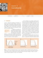
For some conditions we can recognize an optimum concen-
tration or level at which an organism performs best, with its activ-
ity tailing off at both lower and higher levels (Figure 2.1a). But
we need to define what we mean by ‘performs best’. From an
evolutionary point of view, ‘optimal’ conditions are those under
which individuals leave most descendants (are fittest), but these
are often impossible to determine in practice because measures
of fitness should be made over several generations. Instead, we
more often measure the effect of conditions on some key prop-
erty like the activity of an enzyme, the respiration rate of a tissue,
the growth rate of individuals or their rate of reproduction.
However, the effect of variation in conditions on these various
properties will often not be the same; organisms can usually

survive over a wider range of conditions than permit them to
grow or reproduce (Figure 2.1a).
The precise shape of a species’ response will vary from con-
dition to condition. The generalized form of response, shown in
Figure 2.1a, is appropriate for conditions like temperature and pH
conditions may be
altered – but not
consumed
Performance of species
Intensity of condition
Reproduction
Individual
growth
Individual
survival
RR
GG
S
S
(a)
(b)
R
G
S
(c)
R
G
S
Figure 2.1 Response curves illustrating the effects of a range of environmental conditions on individual survival (S), growth (G) and
reproduction (R). (a) Extreme conditions are lethal; less extreme conditions prevent growth; only optimal conditions allow reproduction.

(b) The condition is lethal only at high intensities; the reproduction–growth–survival sequence still applies. (c) Similar to (b), but the
condition is required by organisms, as a resource, at low concentrations.
Chapter 2
Conditions
EIPC02 10/24/05 1:44 PM Page 30
CONDITIONS 31
in which there is a continuum from an adverse or lethal level (e.g.
freezing or very acid conditions), through favorable levels of the
condition to a further adverse or lethal level (heat damage or very
alkaline conditions). There are, though, many environmental con-
ditions for which Figure 2.1b is a more appropriate response curve:
for instance, most toxins, radioactive emissions and chemical
pollutants, where a low-level intensity or concentration of the
condition has no detectable effect, but an increase begins to
cause damage and a further increase may be lethal. There is also
a different form of response to conditions that are toxic at high
levels but essential for growth at low levels (Figure 2.1c). This is
the case for sodium chloride – an essential resource for animals
but lethal at high concentrations – and for the many elements that
are essential micronutrients in the growth of plants and animals
(e.g. copper, zinc and manganese), but that can become lethal
at the higher concentrations sometimes caused by industrial
pollution.
In this chapter, we consider responses to temperature in
much more detail than other conditions, because it is the single
most important condition that affects the lives of organisms, and
many of the generalizations that we make have widespread
relevance. We move on to consider a range of other conditions,
before returning, full circle, to temperature because of the effects
of other conditions, notably pollutants, on global warming. We

begin, though, by explaining the framework within which each
of these conditions should be understood here: the ecological
niche.
2.2 Ecological niches
The term ecological niche is frequently misunderstood and misused.
It is often used loosely to describe the sort of place in which an
organism lives, as in the sentence: ‘Woodlands are the niche of
woodpeckers’. Strictly, however, where an organism lives is its
habitat. A niche is not a place but an idea: a summary of the organ-
ism’s tolerances and requirements. The habitat of a gut micro-
organism would be an animal’s alimentary canal; the habitat of an
aphid might be a garden; and the habitat of a fish could be a whole
lake. Each habitat, however, provides many different niches:
many other organisms also live in the gut, the garden or the lake
– and with quite different lifestyles. The word niche began to gain
its present scientific meaning when Elton wrote in 1933 that the
niche of an organism is its mode of life ‘in the sense that we speak
of trades or jobs or professions in a human community’. The niche
of an organism started to be used to describe how, rather than
just where, an organism lives.
The modern concept of the niche
was proposed by Hutchinson in 1957 to
address the ways in which tolerances and
requirements interact to define the conditions (this chapter) and
resources (Chapter 3) needed by an individual or a species in order
to practice its way of life. Temperature, for instance, limits the
growth and reproduction of all organisms, but different organ-
isms tolerate different ranges of temperature. This range is one
dimension of an organism’s ecological niche. Figure 2.2a shows how
species of plants vary in this dimension of their niche: how they

vary in the range of temperatures at which they can survive. But
there are many such dimensions of a species’ niche – its toler-
ance of various other conditions (relative humidity, pH, wind speed,
water flow and so on) and its need for various resources. Clearly
the real niche of a species must be multidimensional.
It is easy to visualize the early
stages of building such a multidimen-
sional niche. Figure 2.2b illustrates the
way in which two niche dimensions
(temperature and salinity) together define a two-dimensional
area that is part of the niche of a sand shrimp. Three dimensions,
such as temperature, pH and the availability of a particular food,
may define a three-dimensional niche volume (Figure 2.2c). In fact,
we consider a niche to be an n-dimensional hypervolume, where n
is the number of dimensions that make up the niche. It is hard
to imagine (and impossible to draw) this more realistic picture.
None the less, the simplified three-dimensional version captures
the idea of the ecological niche of a species. It is defined by the
boundaries that limit where it can live, grow and reproduce, and
it is very clearly a concept rather than a place. The concept has
become a cornerstone of ecological thought.
Provided that a location is characterized by conditions within
acceptable limits for a given species, and provided also that it con-
tains all the necessary resources, then the species can, potentially,
occur and persist there. Whether or not it does so depends on
two further factors. First, it must be able to reach the location,
and this depends in turn on its powers of colonization and the
remoteness of the site. Second, its occurrence may be precluded
by the action of individuals of other species that compete with it
or prey on it.

Usually, a species has a larger eco-
logical niche in the absence of com-
petitors and predators than it has in
their presence. In other words, there are certain combinations of
conditions and resources that can allow a species to maintain a
viable population, but only if it is not being adversely affected
by enemies. This led Hutchinson to distinguish between the fun-
damental and the realized niche. The former describes the overall
potentialities of a species; the latter describes the more limited
spectrum of conditions and resources that allow it to persist, even
in the presence of competitors and predators. Fundamental and
realized niches will receive more attention in Chapter 8, when
we look at interspecific competition.
The remainder of this chapter looks at some of the most
important condition dimensions of species’ niches, starting with
temperature; the following chapter examines resources, which add
further dimensions of their own.
••
niche dimensions
the n-dimensional
hypervolume
fundamental and
realized niches
EIPC02 10/24/05 1:44 PM Page 31
32 CHAPTER 2
2.3 Responses of individuals to temperature
2.3.1 What do we mean by ‘extreme’?
It seems natural to describe certain environmental conditions
as ‘extreme’, ‘harsh’, ‘benign’ or ‘stressful’. It may seem obvious
when conditions are ‘extreme’: the midday heat of a desert, the

cold of an Antarctic winter, the salinity of the Great Salt Lake.
But this only means that these conditions are extreme for us,
given our particular physiological characteristics and tolerances.
To a cactus there is nothing extreme about the desert condi-
tions in which cacti have evolved; nor are the icy fastnesses of
Antarctica an extreme environment for penguins (Wharton,
2002). It is too easy and dangerous for the ecologist to assume
that all other organisms sense the environment in the way
we do. Rather, the ecologist should try to gain a worm’s-eye
or plant’s-eye view of the environment: to see the world as
others see it. Emotive words like harsh and benign, even relat-
ivities such as hot and cold, should be used by ecologists only
with care.
••••
Ranunculus glacialis
Oxyria digyna
Geum reptans
Pinus cembra
Picea abies
Betula pendula
Larix decidua
Picea abies
Larix decidua
Leucojum vernum
Betula pendula
Fagus sylvatica
Taxus baccata
Abies alba
Prunus laurocerasus
Quercus ilex

Olea europaea
Quercus pubescens
Citrus limonum
Temperature (°C)
25
20
15
10
5
Salinity (%)
0 102030405 15253545
2600
2500
2500
1900
1900
1900
1900
900
900
600
600
600
550
530
250
240
240
240
80

(m)
(a) (b)
Temperature (°C)
5 1015202530
100% mortality
50% mortality
Zero mortality
Temperature
pH
(c)
Food available
Figure 2.2 (a) A niche in one dimension. The range of temperatures at which a variety of plant species from the European Alps can
achieve net photosynthesis of low intensities of radiation (70 W m
−2
). (After Pisek et al., 1973.) (b) A niche in two dimensions for the
sand shrimp (Crangon septemspinosa) showing the fate of egg-bearing females in aerated water at a range of temperatures and salinities.
(After Haefner, 1970.) (c) A diagrammatic niche in three dimensions for an aquatic organism showing a volume defined by the
temperature, pH and availability of food.
EIPC02 10/24/05 1:44 PM Page 32
CONDITIONS 33
2.3.2 Metabolism, growth, development and size
Individuals respond to temperature
essentially in the manner shown in
Figure 2.1a: impaired function and
ultimately death at the upper and
lower extremes (discussed in Sec-
tions 2.3.4 and 2.3.6), with a functional range between the
extremes, within which there is an optimum. This is accounted
for, in part, simply by changes in metabolic effectiveness. For each
10°C rise in temperature, for example, the rate of biological enzy-

matic processes often roughly doubles, and thus appears as an
exponential curve on a plot of rate against temperature (Figure 2.3).
The increase is brought about because high temperature increases
the speed of molecular movement and speeds up chemical reac-
tions. The factor by which a reaction changes over a 10°C range
is referred to as a Q
10
: a rough doubling means that Q
10
≈ 2.
For an ecologist, however, effects on
individual chemical reactions are likely
to be less important than effects on rates
of growth (increases in mass), on rates
of development (progression through
lifecycle stages) and on final body size,
since, as we shall discuss much more fully in Chapter 4, these tend
to drive the core ecological activities of survival, reproduction and
movement. And when we plot rates of growth and development
of whole organisms against temperature, there is quite com-
monly an extended range over which there are, at most, only slight
deviations from linearity (Figure 2.4).
When the relationship between
growth or development is effectively
linear, the temperatures experienced by an organism can be
summarized in a single very useful value, the number of ‘day-
degrees’. For instance, Figure 2.4c shows that at 15°C (5.1°C above
a development threshold of 9.9°C) the predatory mite, Amblyseius
californicus, took 24.22 days to develop (i.e. the proportion of its
total development achieved each day was 0.041 (= 1/24.22)), but

it took only 8.18 days to develop at 25°C (15.1°C above the same
threshold). At both temperatures, therefore, development required
123.5 day-degrees (or, more properly, ‘day-degrees above thresh-
old’), i.e. 24.22 × 5.1 = 123.5, and 8.18 × 15.1 = 123.5. This is also
the requirement for development in the mite at other temper-
atures within the nonlethal range. Such organisms cannot be said
to require a certain length of time for development. What they
require is a combination of time and temperature, often referred
to as ‘physiological time’.
Together, the rates of growth and
development determine the final size of
an organism. For instance, for a given
rate of growth, a faster rate of devel-
opment will lead to smaller final size. Hence, if the responses of
growth and development to variations in temperature are not the
same, temperature will also affect final size. In fact, development
usually increases more rapidly with temperature than does growth,
such that, for a very wide range of organisms, final size tends to
decrease with rearing temperature: the ‘temperature–size rule’ (see
Atkinson et al., 2003). An example for single-celled protists (72 data
sets from marine, brackish and freshwater habitats) is shown
in Figure 2.5: for each 1°C increase in temperature, final cell
volume decreased by roughly 2.5%.
These effects of temperature on growth, development and size
may be of practical rather than simply scientific importance.
Increasingly, ecologists are called upon to predict. We may wish
to know what the consequences would be, say, of a 2°C rise in
temperature resulting from global warming (see Section 2.9.2).
Or we may wish to understand the role of temperature in sea-
sonal, interannual and geographic variations in the productivity

of, for example, marine ecosystems (Blackford et al., 2004). We
cannot afford to assume exponential relationships with temper-
ature if they are really linear, nor to ignore the effects of changes
in organism size on their role in ecological communities.
Motivated, perhaps, by this need to
be able to extrapolate from the known
to the unknown, and also simply by a
wish to discover fundamental organiz-
ing principles governing the world
••••
exponential effects
of temperature on
metabolic reactions
effectively linear
effects on rates
of growth and
development
Temperature (°C)
5 1015202530
Oxygen consumption (µl O
2
g
–1
h
–1
)
600
500
400
300

200
100
Figure 2.3 The rate of oxygen consumption of the Colorado
beetle (Leptinotarsa decemineata), which doubles for every 10°C
rise in temperature up to 20°C, but increases less fast at higher
temperatures. (After Marzusch, 1952.)
day-degree concept
temperature–size
rule
‘universal
temperature
dependence’?
EIPC02 10/24/05 1:44 PM Page 33
••
34 CHAPTER 2
around us, there have been attempts to uncover universal rules of
temperature dependence, for metabolism itself and for develop-
ment rates, linking all organisms by scaling such dependences
with aspects of body size (Gillooly et al., 2001, 2002). Others have
suggested that such generalizations may be oversimplified, stress-
ing for example that characteristics of whole organisms, like
growth and development rates, are determined not only by the
temperature dependence of individual chemical reactions, but also
by those of the availability of resources, their rate of diffusion from
the environment to metabolizing tissues, and so on (Rombough,
2003; Clarke, 2004). It may be that there is room for coexistence
between broad-sweep generalizations at the grand scale and the
more complex relationships at the level of individual species that
these generalizations subsume.
2.3.3 Ectotherms and endotherms

Many organisms have a body temperature that differs little, if
at all, from their environment. A parasitic worm in the gut of
a mammal, a fungal mycelium in the soil and a sponge in the
sea acquire the temperature of the medium in which they live.
Terrestrial organisms, exposed to the sun and the air, are differ-
ent because they may acquire heat directly by absorbing solar radi-
ation or be cooled by the latent heat of evaporation of water (typical
••
Growth rate (µm day
–1
)
–0.2
4
1.0
Temperature (°C)
0.8
246 8 10 12 14 16 18 20 22
(a)
0.6
0.4
0.2
0.0
Developmental rate
0
5
0.25
Temperature (°C)
0.2
0.15
0.1

0.05
3510 20 30
(c)
15 25
y = 0.0081x – 0.05
R
2
= 0.6838
Developmental rate
0.08
18
0.2
Temperature (°C)
0.18
0.16
2820 22 24 26
(b)
0.14
0.12
0.1
y = 0.0124x – 0.1384
R
2
= 0.9753
y = 0.072x – 0.32
R
2
= 0.64
Figure 2.4 Effectively linear relationships between rates of
growth and development and temperature. (a) Growth of the

protist Strombidinopsis multiauris. (After Montagnes et al., 2003.)
(b) Egg development in the beetle Oulema duftschmidi. (After
Severini et al., 2003.) (c) Egg to adult development in the mite
Amblyseius californicus. (After Hart et al., 2002.) The vertical scales
in (b) and (c) represent the proportion of total development
achieved in 1 day at the temperature concerned.
(Difference from V
15
)/V
15
–0.8
–20
1.2
Temperature (°C – 15)
20–10 0 10
0.8
0.4
0
–0.4
Figure 2.5 The temperature–size rule (final size decreases
with increasing temperature) illustrated in protists (65 data sets
combined). The horizontal scale measures temperature as a
deviation from 15°C. The vertical scale measures standardized
size: the difference between the cell volume observed and the cell
volume at 15°C, divided by cell volume at 15°C. The slope of the
mean regression line, which must pass through the point (0,0), was
−0.025 (SE, 0.004); the cell volume decreased by 2.5% for every
1°C rise in rearing temperature. (After Atkinson et al., 2003.)
EIPC02 10/24/05 1:44 PM Page 34
••

CONDITIONS 35
pathways of heat exchange are shown in Figure 2.6). Various fixed
properties may ensure that body temperatures are higher (or lower)
than the ambient temperatures. For example, the reflective,
shiny or silvery leaves of many desert plants reflect radiation that
might otherwise heat the leaves. Organisms that can move have
further control over their body temperature because they can seek
out warmer or cooler environments, as when a lizard chooses to
warm itself by basking on a hot sunlit rock or escapes from the
heat by finding shade.
Amongst insects there are examples of body temperatures raised
by controlled muscular work, as when bumblebees raise their body
temperature by shivering their flight muscles. Social insects such
as bees and termites may combine to control the temperature of
their colonies and regulate them with remarkable thermostatic
precision. Even some plants (e.g. Philodendron) use metabolic heat
to maintain a relatively constant temperature in their flowers;
and, of course, birds and mammals use metabolic heat almost
all of the time to maintain an almost perfectly constant body
temperature.
An important distinction, therefore, is between endotherms
that regulate their temperature by the production of heat within
their own bodies, and ectotherms that rely on external sources of
heat. But this distinction is not entirely clear cut. As we have noted,
apart from birds and mammals, there are also other taxa that use
heat generated in their own bodies to regulate body temperature,
but only for limited periods; and there are some birds and
mammals that relax or suspend their endothermic abilities at the
most extreme temperatures. In particular, many endothermic
animals escape from some of the costs of endothermy by

hibernating during the coldest seasons:
at these times they behave almost like
ectotherms.
Birds and mammals usually maintain
a constant body temperature between
35 and 40°C, and they therefore tend to lose heat in most envir-
onments; but this loss is moderated by insulation in the form of
fur, feathers and fat, and by controlling blood flow near the skin
surface. When it is necessary to increase the rate of heat loss, this
too can be achieved by the control of surface blood flow and
by a number of other mechanisms shared with ectotherms like
panting and the simple choice of an appropriate habitat. Together,
all these mechanisms and properties give endotherms a powerful
(but not perfect) capability for regulating their body temperature,
and the benefit they obtain from this is a constancy of near-optimal
performance. But the price they pay is a large expenditure of energy
(Figure 2.7), and thus a correspondingly large requirement for food
to provide that energy. Over a certain temperature range (the
thermoneutral zone) an endotherm consumes energy at a basal
rate. But at environmental temperatures further and further above
or below that zone, the endotherm consumes more and more
energy in maintaining a constant body temperature. Even in the
thermoneutral zone, though, an endotherm typically consumes
energy many times more rapidly than an ectotherm of compar-
able size.
The responses of endotherms and ectotherms to changing tem-
peratures, then, are not so different as they may at first appear
to be. Both are at risk of being killed by even short exposures to
very low temperatures and by more prolonged exposure to
moderately low temperatures. Both have an optimal environmental

temperature and upper and lower lethal limits. There are also costs
to both when they live at temperatures that are not optimal. For
the ectotherm these may be slower growth and reproduction, slow
movement, failure to escape predators and a sluggish rate of search
for food. But for the endotherm, the maintenance of body tem-
perature costs energy that might have been used to catch more
prey, produce and nurture more offspring or escape more pre-
dators. There are also costs of insulation (e.g. blubber in whales, fur
in mammals) and even costs of changing the insulation between
••
Reradiation
Evaporative
exchange
Radiation
exchange
Radiation
from atomsphere
Reflected
sunlight
Scattered
radiation
Direct radiation
Convective
exchange
Reflected
radiation
Metabolism
Wind
Conduction
exchange

Figure 2.6 Schematic diagram of the
avenues of heat exchange between an
ectotherm and a variety of physical aspects
of its environment. (After Tracy, 1976;
from Hainsworth, 1981.)
endotherms:
temperature regulation
– but at a cost
EIPC02 10/24/05 1:44 PM Page 35
36 CHAPTER 2
seasons. Temperatures only a few degrees higher than the
metabolic optimum are liable to be lethal to endotherms as well
as ectotherms (see Section 2.3.6).
It is tempting to think of ecto-
therms as ‘primitive’ and endotherms as
having gained ‘advanced’ control over
their environment, but it is difficult to
justify this view. Most environments
on earth are inhabited by mixed communities of endothermic and
ectothermic animals. This includes some of the hottest – e.g. desert
rodents and lizards – and some of the coldest – penguins and whales
together with fish and krill at the edge of the Antarctic ice sheet.
Rather, the contrast, crudely, is between the high cost–high benefit
strategy of endotherms and the low cost–low benefit strategy of
ectotherms. But their coexistence tells us that both strategies, in
their own ways, can ‘work’.
2.3.4 Life at low temperatures
The greater part of our planet is below 5°C: ‘cold is the fiercest
and most widespread enemy of life on earth’ (Franks et al., 1990).
More than 70% of the planet is covered with seawater: mostly

deep ocean with a remarkably constant temperature of about 2°C.
If we include the polar ice caps, more than 80% of earth’s bio-
sphere is permanently cold.
By definition, all temperatures below
the optimum are harmful, but there is
usually a wide range of such temperatures that cause no physi-
cal damage and over which any effects are fully reversible. There
are, however, two quite distinct types of damage at low temper-
atures that can be lethal, either to tissues or to whole organisms:
chilling and freezing. Many organisms are damaged by exposure to
temperatures that are low but above freezing point – so-called
••••
Oxygen consumption
40
0
0
5
20
Ambient temperature (°C)
(b)
4
3
2
1
bt
Heat production (cal g
–1
h
–1
)

403010
0
0
40
20
Environmental temperature (°C)
(a)
35
30
25
20
15
10
5
bc
a
45
40
35
30
Body temperature (°C)
10 30
Figure 2.7 (a) Thermostatic heat production by an endotherm is constant in the thermoneutral zone, i.e. between b, the lower
critical temperature, and c, the upper critical temperature. Heat production rises, but body temperature remains constant, as
environmental temperature declines below b, until heat production reaches a maximum possible rate at a low environmental
temperature. Below a, heat production and body temperature both fall. Above c, metabolic rate, heat production and body
temperature all rise. Hence, body temperature is constant at environmental temperatures between a and c. (After Hainsworth, 1981.)
(b) The effect of environmental temperature on the metabolic rate (rate of oxygen consumption) of the eastern chipmunk
(Tamias striatus). bt, body temperature. Note that at temperatures between 0 and 30°C oxygen consumption decreases
approximately linearly as the temperature increases. Above 30°C a further increase in temperature has little effect until

near the animal’s body temperature when oxygen consumption increases again. (After Neumann, 1967; Nedgergaard &
Cannon, 1990.)
ectotherms and
endotherms coexist:
both strategies ‘work’
chilling injury
EIPC02 10/24/05 1:44 PM Page 36
CONDITIONS 37
‘chilling injury’. The fruits of the banana blacken and rot after
exposure to chilling temperatures and many tropical rainforest
species are sensitive to chilling. The nature of the injury is
obscure, although it seems to be associated with the breakdown
of membrane permeability and the leakage of specific ions such
as calcium (Minorsky, 1985).
Temperatures below 0°C can have lethal physical and chem-
ical consequences even though ice may not be formed. Water may
‘supercool’ to temperatures at least as low as −40°C, remaining
in an unstable liquid form in which its physical properties change
in ways that are bound to be biologically significant: its viscosity
increases, its diffusion rate decreases and its degree of ionization
of water decreases. In fact, ice seldom forms in an organism until
the temperature has fallen several degrees below 0°C. Body
fluids remain in a supercooled state until ice forms suddenly around
particles that act as nuclei. The concentration of solutes in the
remaining liquid phase rises as a consequence. It is very rare for
ice to form within cells and it is then inevitably lethal, but the
freezing of extracellular water is one of the factors that prevents
ice forming within the cells themselves (Wharton, 2002), since
water is withdrawn from the cell, and solutes in the cytoplasm
(and vacuoles) become more concentrated. The effects of freez-

ing are therefore mainly osmoregulatory: the water balance of the
cells is upset and cell membranes are destabilized. The effects are
essentially similar to those of drought and salinity.
Organisms have at least two differ-
ent metabolic strategies that allow
survival through the low temperatures
of winter. A ‘freeze-avoiding’ strategy
uses low-molecular-weight polyhydric alcohols (polyols, such as
glycerol) that depress both the freezing and the supercooling point
and also ‘thermal hysteresis’ proteins that prevent ice nuclei
from forming (Figure 2.8a, b). A contrasting ‘freeze-tolerant’
strategy, which also involves the formation of polyols, encour-
ages the formation of extracellular ice, but protects the cell
membranes from damage when water is withdrawn from the cells
(Storey, 1990). The tolerances of organisms to low temperatures
are not fixed but are preconditioned by the experience of tem-
peratures in their recent past. This process is called acclimation
when it occurs in the laboratory and acclimatization when it
occurs naturally. Acclimatization may start as the weather
becomes colder in the fall, stimulating the conversion of almost
the entire glycogen reserve of animals into polyols (Figure 2.8c),
but this can be an energetically costly affair: about 16% of the
carbohydrate reserve may be consumed in the conversion of the
glycogen reserves to polyols.
The exposure of an individual for
several days to a relatively low tem-
perature can shift its whole temperature
response downwards along the tem-
perature scale. Similarly, exposure to a high temperature can shift
the temperature response upwards. Antarctic springtails (tiny

arthropods), for instance, when taken from ‘summer’ temperat-
ures in the field (around 5°C in the Antarctic) and subjected to
a range of acclimation temperatures, responded to temperatures
in the range +2°C to −2°C (indicative of winter) by showing a
marked drop in the temperature at which they froze (Figure 2.9);
but at lower acclimation temperatures still (−5°C, −7°C), they
showed no such drop because the temperatures were themselves
too low for the physiological processes required to make the
acclimation response.
Acclimatization aside, individuals commonly vary in their
temperature response depending on the stage of development they
have reached. Probably the most extreme form of this is when
an organism has a dormant stage in its life cycle. Dormant stages
are typically dehydrated, metabolically slow and tolerant of
extremes of temperature.
2.3.5 Genetic variation and the evolution of
cold tolerance
Even within species there are often differences in temperature
response between populations from different locations, and
these differences have frequently been found to be the result
of genetic differences rather than being attributable solely to
acclimatization. Powerful evidence that cold tolerance varies
between geographic races of a species comes from a study of the
cactus, Opuntia fragilis. Cacti are generally species of hot dry
habitats, but O. fragilis extends as far north as 56°N and at
one site the lowest extreme minimum temperature recorded
was −49.4°C. Twenty populations were sampled from diverse
localities in northern USA and Canada, and were tested for
freezing tolerance and ability to acclimate to cold. Individuals
from the most freeze-tolerant population (from Manitoba)

tolerated −49°C in laboratory tests and acclimated by 19.9°C,
whereas plants from a population in the more equable climate of
Hornby Island, British Columbia, tolerated only −19°C and
acclimated by only 12.1°C (Loik & Nobel, 1993).
There are also striking cases where the geographic range of
a crop species has been extended into colder regions by plant
breeders. Programs of deliberate selection applied to corn (Zea
mays) have expanded the area of the USA over which the crop
can be profitably grown. From the 1920s to the 1940s, the pro-
duction of corn in Iowa and Illinois increased by around 24%,
whereas in the colder state of Wisconsin it increased by 54%.
If deliberate selection can change the tolerance and distribu-
tion of a domesticated plant we should expect natural selection
to have done the same thing in nature. To test this, the plant
Umbilicus rupestris, which lives in mild maritime areas of Great
Britain, was deliberately grown outside its normal range (Wood-
ward, 1990). A population of plants and seeds was taken from a
donor population in the mild-wintered habitat of Cardiff in the
west and introduced in a cooler environment at an altitude of
••••
freeze-avoidance and
freeze-tolerance
acclimation and
acclimatization
EIPC02 10/24/05 1:44 PM Page 37
•• ••
38 CHAPTER 2
Temperature (°C)
–40
–20

0
20
(b)
DecOctSep Nov AprMarFebJan
Glycerol concentration (µmol g
–1
)
0
1000
2000
3000
(a)
DecOctSep Nov AprMarFebJan
Glycogen concentration (µmol g
–1
)
0
400
800
1200
(c)
DecOctSep Nov AprMarFebJan
Month
Figure 2.8 (a) Changes in the glycerol
concentration per gram wet mass of the
freeze-avoiding larvae of the goldenrod gall
moth, Epiblema scudderiana. (b) The daily
temperature maxima and minima (above)
and whole larvae supercooling points
(below) over the same period. (c) Changes

in glycogen concentration over the same
period. (After Rickards et al., 1987.)
EIPC02 10/24/05 1:44 PM Page 38
••
CONDITIONS 39
157 m in Sussex in the south. After 8 years, the temperature
response of seeds from the donor and the introduced populations
had diverged quite strikingly (Figure 2.10a), and subfreezing
temperatures that kill in Cardiff (−12°C) were then tolerated
by 50% of the Sussex population (Figure 2.10b). This suggests
that past climatic changes, for example ice ages, will have changed
the temperature tolerance of species as well as forcing their
migration.
••
–6
–10
–14
–22
Supercooling point (°C)
Exposure temperature (°C)
1
–20
5–3–7
–8
–12
–18
–16
–5–13
Figure 2.9 Acclimation to low
temperatures. Samples of the Antarctic

springtail Cryptopygus antarcticus were taken
from field sites in the summer (c. 5°C) on
a number of days and their supercooling
point (at which they froze) was determined
either immediately (
᭹) or after a period of
acclimation (
᭹) at the temperatures shown.
The supercooling points of the controls
themselves varied because of temperature
variations from day to day, but acclimation
at temperatures in the range +2 to −2°C
(indicative of winter) led to a drop in the
supercooling point, whereas no such drop
was observed at higher temperatures
(indicative of summer) or lower
temperatures (too low for a physiological
acclimation response). Bars are standard
errors. (After Worland & Convey, 2001.)
Germination (%)
2216
0
6
40
80
10
Temperature (°C)
(a)
2
1

Survival (%)
–14–8
0
40
80
–4
Minimum temperature (°C)
(b)
2
–12
1
Figure 2.10 Changes in the behavior of populations of the plant Umbilicus rupestris, established for a period of 8 years in a cool
environment in Sussex from a donor population in a mild-wintered area in South Wales (Cardiff, UK). (a) Temperature responses of
seed germination: (1) responses of samples from the donor population (Cardiff ) in 1978, and (2) responses from the Sussex population in
1987. (b) The low-temperature survival of the donor population at Cardiff, 1978 (1) and of the established population in Sussex, 1987 (2).
(After Woodward, 1990.)
EIPC02 10/24/05 1:44 PM Page 39
40 CHAPTER 2
2.3.6 Life at high temperatures
Perhaps the most important thing about dangerously high
temperatures is that, for a given organism, they usually lie only
a few degrees above the metabolic optimum. This is largely an
unavoidable consequence of the physicochemical properties of most
enzymes (Wharton, 2002). High temperatures may be dangerous
because they lead to the inactivation or even the denaturation of
enzymes, but they may also have damaging indirect effects by lead-
ing to dehydration. All terrestrial organisms need to conserve water,
and at high temperatures the rate of water loss by evaporation
can be lethal, but they are caught between the devil and the deep
blue sea because evaporation is an important means of reducing

body temperature. If surfaces are protected from evaporation (e.g.
by closing stomata in plants or spiracles in insects) the organisms
may be killed by too high a body temperature, but if their sur-
faces are not protected they may die of desiccation.
Death Valley, California, in the
summer, is probably the hottest place
on earth in which higher plants make
active growth. Air temperatures during
the daytime may approach 50°C and soil surface temperatures may
be very much higher. The perennial plant, desert honeysweet
(Tidestromia oblongifolia), grows vigorously in such an environment
despite the fact that its leaves are killed if they reach the same
temperature as the air. Very rapid transpiration keeps the temper-
ature of the leaves at 40–45°C, and in this range they are capable
of extremely rapid photosynthesis (Berry & Björkman, 1980).
Most of the plant species that live in very hot environments
suffer severe shortage of water and are therefore unable to use
the latent heat of evaporation of water to keep leaf temperatures
down. This is especially the case in desert succulents in which water
loss is minimized by a low surface to volume ratio and a low
frequency of stomata. In such plants the risk of overheating
may be reduced by spines (which shade the surface of a cactus)
or hairs or waxes (which reflect a high proportion of the incident
radiation). Nevertheless, such species experience and tolerate
temperatures in their tissues of more than 60°C when the air tem-
perature is above 40°C (Smith et al., 1984).
Fires are responsible for the highest
temperatures that organisms face on
earth and, before the fire-raising activ-
ities of humans, were caused mainly by lightning strikes. The

recurrent risk of fire has shaped the species composition of
arid and semiarid woodlands in many parts of the world. All
plants are damaged by burning but it is the remarkable powers
of regrowth from protected meristems on shoots and seeds that
allow a specialized subset of species to recover from damage and
form characteristic fire floras (see, for example, Hodgkinson, 1992).
Decomposing organic matter in heaps of farmyard manure,
compost heaps and damp hay may reach very high temperatures.
Stacks of damp hay are heated to temperatures of 50–60°C by
the metabolism of fungi such as Aspergillus fumigatus, carried fur-
ther to approximately 65°C by other thermophilic fungi such as
Mucor pusillus and then a little further by bacteria and actinomycetes.
Biological activity stops well short of 100°C but autocom-
bustible products are formed that cause further heating, drive off
water and may even result in fire. Another hot environment
is that of natural hot springs and in these the microbe Thermus
aquaticus grows at temperatures of 67°C and tolerates temper-
atures up to 79°C. This organism has also been isolated from
domestic hot water systems. Many (perhaps all) of the extremely
thermophilic species are prokaryotes. In environments with very
high temperatures the communities contain few species. In gen-
eral, animals and plants are the most sensitive to heat followed
by fungi, and in turn by bacteria, actinomycetes and archaebacteria.
This is essentially the same order as is found in response to many
other extreme conditions, such as low temperature, salinity,
metal toxicity and desiccation.
An ecologically very remarkable
hot environment was first described
only towards the end of the last century.
In 1979, a deep oceanic site was dis-

covered in the eastern Pacific at which
fluids at high temperatures (‘smokers’) were vented from the
sea floor forming thin-walled ‘chimneys’ of mineral materials.
Since that time many more vent sites have been discovered at
mid-ocean crests in both the Atlantic and Pacific Oceans. They
lie 2000–4000 m below sea level at pressures of 200–400 bars
(20–40 MPa). The boiling point of water is raised to 370°C at
200 bars and to 404°C at 400 bars. The superheated fluid emerges
from the chimneys at temperatures as high as 350°C, and as it
cools to the temperature of seawater at about 2°C it provides a
continuum of environments at intermediate temperatures.
Environments at such extreme pressures and temperatures
are obviously extraordinarily difficult to study in situ and in
most respects impossible to maintain in the laboratory. Some
thermophilic bacteria collected from vents have been cultured
successfully at 100°C at only slightly above normal barometric
pressures ( Jannasch & Mottl, 1985), but there is much circumstantial
evidence that some microbial activity occurs at much higher
temperatures and may form the energy resource for the warm
water communities outside the vents. For example, particulate
DNA has been found in samples taken from within the ‘smokers’
at concentrations that point to intact bacteria being present at
temperatures very much higher than those conventionally thought
to place limits on life (Baross & Deming, 1995).
There is a rich eukaryotic fauna in the local neighborhood of
vents that is quite atypical of the deep oceans in general. At one
vent in Middle Valley, Northeast Pacific, surveyed photographic-
ally and by video, at least 55 taxa were documented of which
15 were new or probably new species ( Juniper et al., 1992). There
can be few environments in which so complex and specialized

a community depends on so localized a special condition. The
••••
thermal vents
and other hot
environments
high temperature
and water loss
fire
EIPC02 10/24/05 1:44 PM Page 40
CONDITIONS 41
closest known vents with similar conditions are 2500 km distant.
Such communities add a further list to the planet’s record of species
richness. They present tantalizing problems in evolution and
daunting problems for the technology needed to observe, record
and study them.
2.3.7 Temperature as a stimulus
We have seen that temperature as a condition affects the rate
at which organisms develop. It may also act as a stimulus,
determining whether or not the organism starts its development
at all. For instance, for many species of temperate, arctic and alpine
herbs, a period of chilling or freezing (or even of alternating
high and low temperatures) is necessary before germination will
occur. A cold experience (physiological evidence that winter has
passed) is required before the plant can start on its cycle of
growth and development. Temperature may also interact with
other stimuli (e.g. photoperiod) to break dormancy and so
time the onset of growth. The seeds of the birch (Betula
pubescens) require a photoperiodic stimulus (i.e. experience of a
particular regime of day length) before they will germinate, but if
the seed has been chilled it starts growth without a light stimulus.

2.4 Correlations between temperature and
the distribution of plants and animals
2.4.1 Spatial and temporal variations in temperature
Variations in temperature on and within the surface of the earth
have a variety of causes: latitudinal, altitudinal, continental, sea-
sonal, diurnal and microclimatic effects and, in soil and water, the
effects of depth.
Latitudinal and seasonal variations cannot really be separated.
The angle at which the earth is tilted relative to the sun changes
with the seasons, and this drives some of the main temperature
differentials on the earth’s surface. Superimposed on these broad
geographic trends are the influences of altitude and ‘continentality’.
There is a drop of 1°C for every 100 m increase in altitude in
dry air, and a drop of 0.6°C in moist air. This is the result of the
‘adiabatic’ expansion of air as atmospheric pressure falls with increas-
ing altitude. The effects of continentality are largely attributable
to different rates of heating and cooling of the land and the sea.
The land surface reflects less heat than the water, so the surface
warms more quickly, but it also loses heat more quickly. The sea
therefore has a moderating, ‘maritime’ effect on the temperatures
of coastal regions and especially islands; both daily and seasonal
variations in temperature are far less marked than at more
inland, continental locations at the same latitude. Moreover,
there are comparable effects within land masses: dry, bare areas
like deserts suffer greater daily and seasonal extremes of temperature
than do wetter areas like forests. Thus, global maps of tempera-
ture zones hide a great deal of local variation.
It is much less widely appreciated
that on a smaller scale still there can be
a great deal of microclimatic variation.

For example, the sinking of dense, cold
air into the bottom of a valley at night can make it as much as
30°C colder than the side of the valley only 100 m higher; the
winter sun, shining on a cold day, can heat the south-facing side
of a tree (and the habitable cracks and crevices within it) to as
high as 30°C; and the air temperature in a patch of vegetation
can vary by 10°C over a vertical distance of 2.6 m from the soil
surface to the top of the canopy (Geiger, 1955). Hence, we need
not confine our attention to global or geographic patterns when
seeking evidence for the influence of temperature on the distri-
bution and abundance of organisms.
Long-term temporal variations in
temperature, such as those associated
with the ice ages, were discussed in the previous chapter.
Between these, however, and the very obvious daily and seasonal
changes that we are all aware of, a number of medium-term
patterns have become increasingly apparent. Notable amongst
these are the El Niño-Southern Oscillation (ENSO) and the
North Atlantic Oscillation (NAO) (Figure 2.11) (see Stenseth et
al., 2003). The ENSO originates in the tropical Pacific Ocean off
the coast of South America and is an alternation (Figure 2.11a)
between a warm (El Niño) and a cold (La Niña) state of the water
there, though it affects temperature, and the climate generally,
in terrestrial and marine environments throughout the whole Pacific
basin (Figure 2.11b; for color, see Plate 2.1, between pp. 000 and
000) and beyond. The NAO refers to a north–south alternation
in atmospheric mass between the subtropical Atlantic and the Arctic
(Figure 2.11c) and again affects climate in general rather than
just temperature (Figure 2.11d; for color, see Plate 2.2, between
pp. 000 and 000). Positive index values (Figure 2.11c) are associ-

ated, for example, with relatively warm conditions in North
America and Europe and relatively cool conditions in North
Africa and the Middle East. An example of the effect of NAO
variation on species abundance, that of cod, Gadus morhua, in the
Barents Sea, is shown in Figure 2.12.
2.4.2 Typical temperatures and distributions
There are very many examples of
plant and animal distributions that are
strikingly correlated with some aspect of environmental temper-
ature even at gross taxonomic and systematic levels (Figure 2.13).
At a finer scale, the distributions of many species closely match
maps of some aspect of temperature. For example, the northern
limit of the distribution of wild madder plants (Rubia peregrina)
is closely correlated with the position of the January 4.5°C
••••
microclimatic
variation
ENSO and NAO
isotherms
EIPC02 10/24/05 1:44 PM Page 41
••••
42 CHAPTER 2
–2
1950 1955 1960 1965 1970 1975 1980 1985 1990 1995
Year
2000
Niño 3.4 region (threshold − 0°C)
2
1
0

–1
Sea surface temperature anomalies
3
(a)
Figure 2.11 (a) The El Niño–Southern Oscillation (ENSO) from 1950 to 2000 as measured by sea surface temperature anomalies
(differences from the mean) in the equatorial mid-Pacific. The El Niño events (> 0.4°C above the mean) are shown in dark color,
and the La Niña events (> 0.4°C below the mean) are shown in pale color. (Image from http:
/
/www.cgd.ucar.edu/cas/catalog/
climind/Nino
_
3
_
3.4
_
indices.html.) (b) Maps of examples of El Niño (November 1997) and La Niña (February 1999) events in terms
of sea height above average levels. Warmer seas are higher; for example, a sea height 15–20 cm below average equates to a temperature
anomaly of approximately 2–3°C. (Image from http:
//topex-www.jpl.nasa.gov/science/images/el-nino-la-nina.jpg.) (For color, see
Plate 2.1, between pp. 000 and 000.)
(b)
EIPC02 10/24/05 1:44 PM Page 42
••••
CONDITIONS 43
–4
1860
1880
1900 1920 1940
1960
1980

6
(c)
Year
(L
n
– S
n
)
2000
2
4
0
–2
Figure 2.11 (continued) (c) The North Atlantic Oscillation (NAO) from 1864 to 2003 as measured by the normalized sea-level
pressure difference (L
n
− S
n
) between Lisbon, Portugal and Reykjavik, Iceland. (Image from />nao.stat.winter.html#winter.) (d) Typical winter conditions when the NAO index is positive or negative. Conditions that are more than
usually warm, cold, dry or wet are indicated. (Image from http:
//www.ldeo.columbia.edu/NAO/.) (For color, see Plate 2.2, between
pp. 000 and 000.)
(d)(i)
(d)(ii)
EIPC02 10/24/05 1:44 PM Page 43
44 CHAPTER 2
isotherm (Figure 2.14a; an isotherm is a line on a map joining places
that experience the same temperature – in this case a January mean
of 4.5°C). However, we need to be very careful how we inter-
pret such relationships: they can be extremely valuable in predicting

where we might and might not find a particular species; they
may suggest that some feature related to temperature is import-
ant in the life of the organisms; but they do not prove that tem-
perature causes the limits to a species’ distribution. The literature
relevant to this and many other correlations between temperature
and distribution patterns is reviewed by Hengeveld (1990), who
also describes a more subtle graphical procedure. The minimum
temperature of the coldest month and the maximum temperature
of the hottest month are estimated for many places within and
outside the range of a species. Each location is then plotted on a
graph of maximum against minimum temperature, and a line is
drawn that optimally discriminates between the presence and
absence records (Figure 2.14b). This line is then used to define
the geographic margin of the species distributions (Figure 2.14c).
This may have powerful predictive value, but it still tells us
nothing about the underlying forces that cause the distribution
patterns.
One reason why we need to be cautious about reading too
much into correlations of species distributions with maps of tem-
perature is that the temperatures measured for constructing
isotherms for a map are only rarely those that the organisms expe-
rience. In nature an organism may choose to lie in the sun or hide
••••
log(abundance age 3 in 1000s)
4.5
–5
8.0
NAO index
7.5
7.0

6.5
6.0
5.5
5.0
6–4–3–2–1012345
log(abundance age 3 in 1000s)
4.5
50
8.0
Length of 5-month-old cod (mm)
7.5
7.0
6.5
6.0
5.5
5.0
10060 70 80 90
Temperature (°C)
2.5
–5
5
NAO index
4.5
4
3.5
3
6–4–3–2–1012345
Length of 5-month-old cod (mm)
50
2.5

100
Temperature (°C)
90
80
70
60
53 3.5 4 4.5
(a)
(d)
(b)
(c)
Figure 2.12 (a) The abundance of 3-year-old cod, Gadus morhua, in the Barents Sea is positively correlated with the value of the North
Atlantic Oscillation (NAO) index for that year. The mechanism underlying this correlation is suggested in (b–d). (b) Annual mean
temperature increases with the NAO index. (c) The length of 5-month-old cod increases with annual mean temperature. (d) The
abundance of cod at age 3 increases with their length at 5 months. (After Ottersen et al., 2001.)
EIPC02 10/24/05 1:44 PM Page 44
CONDITIONS 45
in the shade and, even in a single day, may experience a baking
midday sun and a freezing night. Moreover, temperature varies
from place to place on a far finer scale than will usually concern
a geographer, but it is the conditions in these ‘microclimates’ that
will be crucial in determining what is habitable for a particular
species. For example, the prostrate shrub Dryas octopetala is
restricted to altitudes exceeding 650 m in North Wales, UK,
where it is close to its southern limit. But to the north, in
Sutherland in Scotland, where it is generally colder, it is found
right down to sea level.
2.4.3 Distributions and extreme conditions
For many species, distributions are accounted for not so much
by average temperatures as by occasional extremes, especially

occasional lethal temperatures that preclude its existence. For
instance, injury by frost is probably the single most important fac-
tor limiting plant distribution. To take one example: the saguaro
cactus (Carnegiea gigantea) is liable to be killed when temperatures
remain below freezing for 36 h, but if there is a daily thaw it is
under no threat. In Arizona, the northern and eastern edges of
the cactus’ distribution correspond to a line joining places where
on occasional days it fails to thaw. Thus, the saguaro is absent
where there are occasionally lethal conditions – an individual need
only be killed once.
Similarly, there is scarcely any crop
that is grown on a large commercial
scale in the climatic conditions of its wild ancestors, and it is well
known that crop failures are often caused by extreme events, espe-
cially frosts and drought. For instance, the climatic limit to the
geographic range for the production of coffee (Coffea arabica and
C. robusta) is defined by the 13°C isotherm for the coldest month
of the year. Much of the world’s crop is produced in the high-
land microclimates of the São Paulo and Paraná districts of
••••
Number of families
200–40–60
100
200
–20
Temperature (°C)
Northern hemisphere
Southern hemisphere
(a)
4.5°C

Temperature in warmest month (°C)
2–8–12
0
–14
10
12
18
–10
Temperature in coldest month (°C)
(b)
–6 –4 –2 0
14
16
(c)
20
Figure 2.13 The relationship between absolute minimum
temperature and the number of families of flowering plants in the
northern and southern hemispheres. (After Woodward, 1987, who
also discusses the limitations to this sort of analysis and how the
history of continental isolation may account for the odd difference
between northern and southern hemispheres.)
Figure 2.14 (a) The northern limit of the distribution of the wild madder (Rubia peregrina) is closely correlated with the position of
the January 4.5°C isotherm. (After Cox et al., 1976.) (b) A plot of places within the range of Tilia cordat (
᭹), and outside its range (7) in
the graphic space defined by the minimum temperature of the coldest month and the maximum temperature of the warmest month.
(c) Margin of the geographic range of T. cordata in northern Europe defined by the straight line in (b). ((b, c) after Hintikka, 1963; from
Hengeveld, 1990.)
you only die once
EIPC02 10/24/05 1:44 PM Page 45
46 CHAPTER 2

Brazil. Here, the average minimum temperature is 20°C, but
occasionally cold winds and just a few hours of temperature
close to freezing are sufficient to kill or severely damage the trees
(and play havoc with world coffee prices).
2.4.4 Distributions and the interaction of temperature
with other factors
Although organisms respond to each condition in their environ-
ment, the effects of conditions may be determined largely by the
responses of other community members. Temperature does not
act on just one species: it also acts on its competitors, prey, para-
sites and so on. This, as we saw in Section 2.2, was the difference
between a fundamental niche (where an organism could live) and
a realized niche (where it actually lived). For example, an organ-
ism will suffer if its food is another species that cannot tolerate
an environmental condition. This is illustrated by the distribution
of the rush moth (Coleophora alticolella) in England. The moth lays
its eggs on the flowers of the rush Juncus squarrosus and the cater-
pillars feed on the developing seeds. Above 600 m, the moths and
caterpillars are little affected by the low temperatures, but the rush,
although it grows, fails to ripen its seeds. This, in turn, limits the
distribution of the moth, because caterpillars that hatch in the colder
elevations will starve as a result of insufficient food (Randall, 1982).
The effects of conditions on disease
may also be important. Conditions
may favor the spread of infection
(winds carrying fungal spores), or favor the growth of the para-
site, or weaken the defenses of the host. For example, during an
epidemic of southern corn leaf blight (Helminthosporium maydis)
in a corn field in Connecticut, the plants closest to the trees
that were shaded for the longest periods were the most heavily

diseased (Figure 2.15).
Competition between species can
also be profoundly influenced by
environmental conditions, especially
temperature. Two stream salmonid fishes, Salvelinus malma and
S. leucomaenis, coexist at intermediate altitudes (and therefore
intermediate temperatures) on Hokkaido Island, Japan, whereas
only the former lives at higher altitudes (lower temperatures)
and only the latter at lower altitudes (see also Section 8.2.1). A
reversal, by a change in temperature, of the outcome of com-
petition between the species appears to play a key role in this.
For example, in experimental streams supporting the two species
maintained at 6°C over a 191-day period (a typical high altitude
temperature), the survival of S. malma was far superior to that of
S. leucomaenis; whereas at 12°C (typical low altitude), both species
survived less well, but the outcome was so far reversed that by
around 90 days all of the S. malma had died (Figure 2.16). Both
species are quite capable, alone, of living at either temperature.
Many of the interactions between
temperature and other physical condi-
tions are so strong that it is not sensi-
ble to consider them separately. The
relative humidity of the atmosphere, for example, is an import-
ant condition in the life of terrestrial organisms because it plays
a major part in determining the rate at which they lose water. In
practice, it is rarely possible to make a clean distinction between
the effects of relative humidity and of temperature. This is simply
because a rise in temperature leads to an increased rate of eva-
poration. A relative humidity that is acceptable to an organism at
a low temperature may therefore be unacceptable at a higher tem-

perature. Microclimatic variations in relative humidity can be even
more marked than those involving temperature. For instance, it
is not unusual for the relative humidity to be almost 100% at ground
level amongst dense vegetation and within the soil, whilst the air
immediately above, perhaps 40 cm away, has a relative humidity
••••
15
10
5
0
1357
Row number from shading trees at edge of field
9111315
Percentage leaf area infected
Figure 2.15 The incidence of southern
corn leaf blight (Helminthosporium maydis)
on corn growing in rows at various
distances from trees that shaded them.
Wind-borne fungal diseases were
responsible for most of this mortality
(Harper, 1955). (From Lukens &
Mullany, 1972.)
disease
competition
temperature and
humidity
EIPC02 10/24/05 1:44 PM Page 46
CONDITIONS 47
of only 50%. The organisms most obviously affected by humid-
ity in their distribution are those ‘terrestrial’ animals that are

actually, in terms of the way they control their water
balance, ‘aquatic’. Amphibians, terrestrial isopods, nematodes,
earthworms and molluscs are all, at least in their active stages,
confined to microenvironments where the relative humidity is at
or very close to 100%. The major group of animals to escape such
confinement are the terrestrial arthropods, especially insects.
Even here though, the evaporative loss of water often confines
their activities to habitats (e.g. woodlands) or times of day (e.g.
dusk) when relative humidity is relatively high.
2.5 pH of soil and water
The pH of soil in terrestrial environments or of water in aquatic
ones is a condition that can exert a powerful influence on the dis-
tribution and abundance of organisms. The protoplasm of the root
cells of most vascular plants is damaged as a direct result of toxic
concentrations of H
+
or OH
−
ions in soils below pH 3 or above
pH 9, respectively. Further, indirect effects occur because soil pH
influences the availability of nutrients and/or the concentration
of toxins (Figure 2.17).
Increased acidity (low pH) may act in three ways: (i) directly,
by upsetting osmoregulation, enzyme activity or gaseous exchange
across respiratory surfaces; (ii) indirectly, by increasing the con-
centration of toxic heavy metals, particularly aluminum (Al
3+
) but
also manganese (Mn
2+

) and iron (Fe
3+
), which are essential plant
nutrients at higher pHs; and (iii) indirectly, by reducing the qual-
ity and range of food sources available to animals (e.g. fungal
growth is reduced at low pH in streams (Hildrew et al., 1984) and
the aquatic flora is often absent or less diverse). Tolerance limits
for pH vary amongst plant species, but only a minority are able
to grow and reproduce at a pH below about 4.5.
In alkaline soils, iron (Fe
3+
) and phosphate (PO
4
3+
), and certain
trace elements such as manganese (Mn
2+
), are fixed in relatively
insoluble compounds, and plants may then suffer because there
is too little rather than too much of them. For example, calcifuge
plants (those characteristic of acid soils) commonly show symp-
toms of iron deficiency when they are transplanted to more alka-
line soils. In general, however, soils and waters with a pH above
7 tend to be hospitable to many more species than those that are
more acid. Chalk and limestone grasslands carry a much richer
flora (and associated fauna) than acid grasslands and the situation
is similar for animals inhabiting streams, ponds and lakes.
Some prokaryotes, especially the Archaebacteria, can tolerate
and even grow best in environments with a pH far outside the
range tolerated by eukaryotes. Such environments are rare, but

occur in volcanic lakes and geothermal springs where they are
••••
1.0
0
Survival rate function
Experiment period (days)
100 200
0.5
0 100 2000
6°C12°C
S. malma
S. leucomaenis
Figure 2.16 Changing temperature
reverses the outcome of competition.
At low temperature (6°C) on the left, the
salmonid fish Salvelinus malma outsurvives
cohabiting S. leucomaenis, whereas at 12°C,
on the right, S. leucomaenis drives S. malma
to extinction. Both species are quite
capable, alone, of living at either
temperature. (After Taniguchi &
Nakano, 2000.)
9645
pH
387
Mo
Fe and Mn
Cu and Zn
K
Ca and Mg

P and B
N and S mobilization
Al
H
+
and OH
–
toxicity
Fgiure 2.17 The toxicity of H
+
and OH
−
to plants, and the
availability to them of minerals (indicated by the widths of
the bands) is influenced by soil pH. (After Larcher, 1980.)
EIPC02 10/24/05 1:44 PM Page 47
48 CHAPTER 2
dominated by sulfur-oxidizing bacteria whose pH optima lie
between 2 and 4 and which cannot grow at neutrality (Stolp, 1988).
Thiobacillus ferroxidans occurs in the waste from industrial metal-
leaching processes and tolerates pH 1; T. thiooxidans cannot only
tolerate but can grow at pH 0. Towards the other end of the
pH range are the alkaline environments of soda lakes with pH
values of 9–11, which are inhabited by cyanobacteria such as
Anabaenopsis arnoldii and Spirulina platensis; Plectonema nostocorum
can grow at pH 13.
2.6 Salinity
For terrestrial plants, the concentration of salts in the soil water
offers osmotic resistance to water uptake. The most extreme saline
conditions occur in arid zones where the predominant movement

of soil water is towards the surface and cystalline salt accumu-
lates. This occurs especially when crops have been grown in
arid regions under irrigation; salt pans then develop and the land
is lost to agriculture. The main effect of salinity is to create the
same kind of osmoregulatory problems as drought and freezing
and the problems are countered in much the same ways. For
example, many of the higher plants that live in saline environ-
ments (halophytes) accumulate electrolytes in their vacuoles, but
maintain a low concentration in the cytoplasm and organelles
(Robinson et al., 1983). Such plants maintain high osmotic pres-
sures and so remain turgid, and are protected from the damaging
action of the accumulated electrolytes by polyols and membrane
protectants.
Freshwater environments present a set of specialized environ-
mental conditions because water tends to move into organisms
from the environment and this needs to be resisted. In marine
habitats, the majority of organisms are isotonic to their environ-
ment so that there is no net flow of water, but there are many
that are hypotonic so that water flows out from the organism to
the environment, putting them in a similar position to terrestrial
organisms. Thus, for many aquatic organisms the regulation of
body fluid concentration is a vital and sometimes an energetically
expensive process. The salinity of an aquatic environment can have
an important influence on distribution and abundance, especially
in places like estuaries where there is a particularly sharp gradi-
ent between truly marine and freshwater habitats.
The freshwater shrimps Palaemonetes pugio and P. vulgaris, for
example, co-occur in estuaries on the eastern coat of the USA
at a wide range of salinities, but the former seems to be more
tolerant of lower salinities than the latter, occupying some

habitats from which the latter is absent. Figure 2.18 shows the
mechanism likely to be underlying this (Rowe, 2002). Over the
low salinity range (though not at the effectively lethal lowest salin-
ity) metabolic expenditure was significantly lower in P. pugio.
P. vulgaris requires far more energy simply to maintain itself,
putting it at a severe disadvantage in competition with P. pugio
even when it is able to sustain such expenditure.
2.6.1 Conditions at the boundary between the sea
and land
Salinity has important effects on the distribution of organisms
in intertidal areas but it does so through interactions with other
conditions – notably exposure to the air and the nature of the
substrate.
••••
Standard metabolic expenditure (J day
–1
)
33
32
31
30
29
28
27
26
25
24
23
22
21

20
19
18
17
Salinity (ppt)
0
1 2 3 4 5 6 7 353025201510
Overall mean,
P. vulgaris (24.85)
Overall mean,
P. pugio (22.91)
P. pugio
P. vulgaris
Figure 2.18 Standard metabolic
expenditure (estimated through minimum
oxygen consumption) in two species of
shrimp, Palaemonetes pugio and P. vulgaris,
at a range of salinities. There was
significant mortality of both species over
the experimental period at 0.5 ppt (parts
per thousand), especially in P. vulgaris (75%
compared with 25%). (After Rowe, 2002.)
EIPC02 10/24/05 1:44 PM Page 48
CONDITIONS 49
Algae of all types have found suitable habitats permanently
immersed in the sea, but permanently submerged higher plants
are almost completely absent. This is a striking contrast with
submerged freshwater habitats where a variety of flowering
plants have a conspicuous role. The main reason seems to be that
higher plants require a substrate in which their roots can find

anchorage. Large marine algae, which are continuously sub-
merged except at extremely low tides, largely take their place
in marine communities. These do not have roots but attach
themselves to rocks by specialized ‘holdfasts’. They are excluded
from regions where the substrates are soft and holdfasts cannot
‘hold fast’. It is in such regions that the few truly marine flower-
ing plants, for example sea grasses such as Zostera and Posidonia,
form submerged communities that support complex animal
communities.
Most species of higher plants that
root in seawater have leaves and shoots
that are exposed to the atmosphere
for a large part of the tidal cycle, such
as mangroves, species of the grass genus Spartina and extreme halo-
phytes such as species of Salicornia that have aerial shoots but whose
roots are exposed to the full salinity of seawater. Where there
is a stable substrate in which plants can root, communities of
flowering plants may extend right through the intertidal zone
in a continuum extending from those continuously immersed in
full-strength seawater (like the sea grasses) through to totally non-
saline conditions. Salt marshes, in particular, encompass a range
of salt concentrations running from full-strength seawater down
to totally nonsaline conditions.
Higher plants are absent from intertidal rocky sea shores
except where pockets of soft substrate may have formed in
crevices. Instead, such habitats are dominated by the algae,
which give way to lichens at and above the high tide level where
the exposure to desiccation is highest. The plants and animals that
live on rocky sea shores are influenced by environmental condi-
tions in a very profound and often particularly obvious way by

the extent to which they tolerate exposure to the aerial environ-
ment and the forces of waves and storms. This expresses itself in
the zonation of the organisms, with different species at different
heights up the shore (Figure 2.19).
The extent of the intertidal zone
depends on the height of tides and the
slope of the shore. Away from the shore, the tidal rise and fall
are rarely greater than 1 m, but closer to shore, the shape of the
land mass can funnel the ebb and flow of the water to produce
extraordinary spring tidal ranges of, for example, nearly 20 m in
the Bay of Fundy (between Nova Scotia and New Brunswick,
Canada). In contrast, the shores of the Mediterranean Sea
••••
Figure 2.19 A general zonation scheme
for the seashore determined by relative
lengths of exposure to the air and to the
action of waves. (After Raffaelli &
Hawkins, 1996.)
Land
Sea
Supralittoral zone
Upper limit of lamination seaweeds
Upper limit of barnacles
Upper limit of periwinkle snails
Supralittoral fringe
Midlittoral zone
Infralittoral
zone
Infralittoral
fringe

Littoral zone
algae and higher
plants
zonation
EIPC02 10/24/05 1:44 PM Page 49
50 CHAPTER 2
experience scarcely any tidal range. On steep shores and rocky
cliffs the intertidal zone is very short and zonation is compressed.
To talk of ‘zonation as a result of exposure’, however, is to
oversimplify the matter greatly (Raffaelli & Hawkins, 1996). In
the first place, ‘exposure’ can mean a variety, or a combination
of, many different things: desiccation, extremes of temperature,
changes in salinity, excessive illumination and the sheer physical
forces of pounding waves and storms (to which we turn in
Section 2.7). Furthermore, ‘exposure’ only really explains the
upper limits of these essentially marine species, and yet zonation
depends on them having lower limits too. For some species
there can be too little exposure in the lower zones. For instance,
green algae would be starved of blue and especially red light
if they were submerged for long periods too low down the
shore. For many other species though, a lower limit to distribu-
tion is set by competition and predation (see, for example, the
discussion in Paine, 1994). The seaweed Fucus spiralis will readily
extend lower down the shore than usual in Great Britain whenever
other competing midshore fucoid seaweeds are scarce.
2.7 Physical forces of winds, waves and currents
In nature there are many forces of the environment that have their
effect by virtue of the force of physical movement – wind and
water are prime examples.
In streams and rivers, both plants and animals face the con-

tinual hazard of being washed away. The average velocity of flow
generally increases in a downstream direction, but the greatest
danger of members of the benthic (bottom-dwelling) community
being washed away is in upstream regions, because the water here
is turbulent and shallow. The only plants to be found in the most
extreme flows are literally ‘low profile’ species like encrusting
and filamentous algae, mosses and liverworts. Where the flow is
slightly less extreme there are plants like the water crowfoot
(Ranunculus fluitans), which is streamlined, offering little resistance
to flow and which anchors itself around an immovable object
by means of a dense development of adventitious roots. Plants
such as the free-floating duckweed (Lemna spp.) are usually only
found where there is negligible flow.
The conditions of exposure on sea shores place severe limits
on the life forms and habits of species that can tolerate repeated
pounding and the suction of wave action. Seaweeds anchored
on rocks survive the repeated pull and push of wave action by
a combination of powerful attachment by holdfasts and extreme
flexibility of their thallus structure. Animals in the same envir-
onment either move with the mass of water or, like the algae,
rely on subtle mechanisms of firm adhesion such as the power-
ful organic glues of barnacles and the muscular feet of limpets.
A comparable diversity of morphological specializations is to
be found amongst the invertebrates that tolerate the hazards of
turbulent, freshwater streams.
2.7.1 Hazards, disasters and catastrophes:
the ecology of extreme events
The wind and the tides are normal daily ‘hazards’ in the life of
many organisms. The structure and behavior of these organisms
bear some witness to the frequency and intensity of such hazards

in the evolutionary history of their species. Thus, most trees with-
stand the force of most storms without falling over or losing their
living branches. Most limpets, barnacles and kelps hold fast to the
rocks through the normal day to day forces of the waves and tides.
We can also recognize a scale of more severely damaging forces
(we might call them ‘disasters’) that occur occasionally, but with
sufficient frequency to have contributed repeatedly to the forces
of natural selection. When such a force recurs it will meet a popu-
lation that still has a genetic memory of the selection that acted
on its ancestors – and may therefore suffer less than they did.
In the woodlands and shrub communities of arid zones, fire has
this quality, and tolerance of fire damage is a clearly evolved
response (see Section 2.3.6).
When disasters strike natural communities it is only rarely
that they have been carefully studied before the event. One
exception is cyclone ‘Hugo’ which struck the Caribbean island
of Guadeloupe in 1994. Detailed accounts of the dense humid
forests of the island had been published only recently before (Ducrey
& Labbé, 1985, 1986). The cyclone devastated the forests with mean
maximum wind velocities of 270 km h
−1
and gusts of 320 km h
−1
.
Up to 300 mm of rain fell in 40 h. The early stages of regenera-
tion after the cyclone (Labbé, 1994) typify the responses of long-
established communities on both land or sea to massive forces
of destruction. Even in ‘undisturbed’ communities there is a con-
tinual creation of gaps as individuals (e.g. trees in a forest, kelps
on a sea shore) die and the space they occupied is recolonized

(see Section 16.7). After massive devastation by cyclones or
other widespread disasters, recolonization follows much the
same course. Species that normally colonize only natural gaps in
the vegetation come to dominate a continuous community.
In contrast to conditions that we have called ‘hazards’ and
‘disasters’ there are natural occurrences that are enormously
damaging, yet occur so rarely that they may have no lasting
selective effect on the evolution of the species. We might call
such events ‘catastrophes’, for example the volcanic eruption of
Mt St Helens or of the island of Krakatau. The next time that
Krakatau erupts there are unlikely to be any genes persisting that
were selected for volcano tolerance!
2.8 Environmental pollution
A number of environmental conditions that are, regrettably,
becoming increasingly important are due to the accumulation of
toxic by-products of human activities. Sulfur dioxide emitted from
power stations, and metals like copper, zinc and lead, dumped
••••
EIPC02 10/24/05 1:44 PM Page 50
CONDITIONS 51
around mines or deposited around refineries, are just some of the
pollutants that limit distributions, especially of plants. Many such
pollutants are present naturally but at low concentrations, and some
are indeed essential nutrients for plants. But in polluted areas their
concentrations can rise to lethal levels. The loss of species is often
the first indication that pollution has occurred, and changes in the
species richness of a river, lake or area of land provide bioassays
of the extent of their pollution (see, for example, Lovett Doust
et al., 1994).
Yet it is rare to find even the most

inhospitable polluted areas entirely
devoid of species; there are usually at
least a few individuals of a few species that can tolerate the con-
ditions. Even natural populations from unpolluted areas often
contain a low frequency of individuals that tolerate the pollutant;
this is part of the genetic variability present in natural populations.
Such individuals may be the only ones to survive or colonize as
pollutant levels rise. They may then become the founders of a
tolerant population to which they have passed on their ‘tolerance’
genes, and, because they are the descendants of just a few founders,
such populations may exhibit notably low genetic diversity overall
(Figure 2.20). Moreover, species themselves may differ greatly in
their ability to tolerate pollutants. Some plants, for example, are
‘hyperaccumulators’ of heavy metals – lead, cadmium and so on
– with an ability not only to tolerate but also to accumulate much
higher concentrations than the norm (Brooks, 1998). As a result,
such plants may have an important role to play in ‘bioremedia-
tion’ (Salt et al., 1998), removing pollutants from the soil so that
eventually other, less tolerant plants can grow there too (discussed
further in Section 7.2.1).
Thus, in very simple terms, a pollutant has a twofold effect.
When it is newly arisen or is at extremely high concentrations,
there will be few individuals of any species present (the exceptions
being naturally tolerant variants or their immediate descendants).
Subsequently, however, the polluted area is likely to support a
much higher density of individuals, but these will be representat-
ives of a much smaller range of species than would be present in
the absence of the pollutant. Such newly evolved, species-poor
communities are now an established part of human environments
(Bradshaw, 1987).

Pollution can of course have its effects far from the original
source (Figure 2.21). Toxic effluents from a mine or a factory may
enter a watercourse and affect its flora and fauna for its whole
length downstream. Effluents from large industrial complexes can
pollute and change the flora and fauna of many rivers and lakes
in a region and cause international disputes.
A striking example is the creation of
‘acid rain’ – for example that falling in
Ireland and Scandinavia from indus-
trial activities in other countries. Since the Industrial Revolution,
the burning of fossil fuels and the consequent emission to the
atmosphere of various pollutants, notably sulfur dioxide, has
produced a deposition of dry acidic particles and rain that is essen-
tially dilute sulfuric acid. Our knowledge of the pH tolerances
of diatom species enables an approximate pH history of a lake to
be constructed. The history of the acidification of lakes is often
••••
Kangaroo Island
Middle Beach
Edinburgh
Port Pirie
BSI
Bond Sharing Index (BSI)/ Matching Index (MI)
1
0.2
0
0.4
0.6
0.8
Increasing genetic diversity

MI (isopod)
(b)
Middle Beach
Port Pirie
LC 50 (multiples of the concentrations of
metals in the substratum at Port Pirie)
WinterSummer
0
10
12
14
8
6
4
2
(a)
Figure 2.20 The response of the marine isopod, Platynympha longicaudata, to pollution around the largest lead smelting operation in
the world, Port Pirie, South Australia. (a) Tolerance, both summer and winter, was significantly higher (P < 0.05) than for animals from
a control (unpolluted) site, as measured by the concentration in food of a combination of metals (lead, copper, cadmium, zinc and
manganese) required to kill 50% of the population (LC50). (b) Genetic diversity at Port Pirie was significantly lower than at three
unpolluted sites, as measured by two indices of diversity based on RAPDs (random amplified polymorphic DNA). (After Ross et al., 2002.)
rare tolerators
acid rain
EIPC02 10/24/05 1:44 PM Page 51
••
52 CHAPTER 2
recorded in the succession of diatom species accumulated in lake
sediments (Flower et al., 1994). Figure 2.22, for example, shows
how diatom species composition has changed in Lough Maam,
Ireland – far from major industrial sites. The percentage of vari-

ous diatom species at different depths reflects the flora present
at various times in the past (four species are illustrated). The age
of layers of sediment can be determined by the radioactive decay
of lead-210 (and other elements). We know the pH tolerance of
the diatom species from their present distribution and this can be
used to reconstruct what the pH of the lake has been in the past.
Note how the waters acidified since about 1900. The diatoms
Fragilaria virescens and Brachysira vitrea have declined markedly dur-
ing this period while the acid-tolerant Cymbella perpusilla and
Frustulia rhomboides increased after 1900.
2.9 Global change
In Chapter 1 we discussed some of the ways in which global
environments have changed over the long timescales involved
in continental drift and the shorter timescales of the repeated
ice ages. Over these timescales some organisms have failed to
accommodate to the changes and have become extinct, others have
migrated so that they continue to experience the same conditions
but in a different place, and it is probable that others have
changed their nature (evolved) and tolerated some of the
changes. We now turn to consider global changes that are occur-
ring in our own lifetimes – consequences of our own activities –
and that are predicted, in most scenarios, to bring about profound
changes in the ecology of the planet.
2.9.1 Industrial gases and the greenhouse effect
A major element of the Industrial Revolution was the switch from
the use of sustainable fuels to the use of coal (and later, oil)
as a source of power. Between the middle of the 19th and the
middle of the 20th century the burning of fossil fuels, together
with extensive deforestation, added about 9 × 10
10

tonnes of carbon
dioxide (CO
2
) to the atmosphere and even more has been added
since. The concentration of CO
2
in the atmosphere before the
Industrial Revolution (measured in gas trapped in ice cores) was
about 280 ppm, a fairly typical interglacial ‘peak’ (Figure 2.23),
but this had risen to around 370 ppm by around the turn of the
millennium and is still rising (see Figure 18.22).
Solar radiation incident on the earth’s atmosphere is in part
reflected, in part absorbed, and part is transmitted through to the
earth’s surface, which absorbs and is warmed by it. Some of this
absorbed energy is radiated back to the atmosphere where atmo-
spheric gases, mainly water vapor and CO
2
absorb about 70% of
it. It is this trapped reradiated energy that heats the atmosphere
in what is called the ‘greenhouse effect’. The greenhouse effect
was of course part of the normal environment before the
Industrial Revolution and carried responsibility for some of
the environmental warmth before industrial activity started to
enhance it. At that time, atmospheric water vapor was respons-
ible for the greater portion of the greenhouse effect.
••
25
10
10
25

100
250
100
25
10
500
1000
100
250
1000
2000
3000
4000
1000
100
250
500
500
2000
1000
500
Figure 2.21 An example of long-distance environmental
pollution. The distribution in Great Britain of fallout of radioactive
caesium (Bq m
−2
) from the Chernobyl nuclear accident in the
Soviet Union in 1986. The map shows the persistence of the
pollutant on acid upland soils where it is recycled through soils,
plants and animals. Sheep in the upland areas contained more
caesium-137 (

137
Cs) in 1987 and 1988 (after recycling) than in 1986.
137
Cs has a half-life of 30 years! On typical lowland soils it is more
quickly immobilized and does not persist in the food chains.
(After NERC, 1990.)
EIPC02 10/24/05 1:44 PM Page 52
••
CONDITIONS 53
In addition to the enhancement
of greenhouse effects by increased
CO
2
, other trace gases have increased
markedly in the atmosphere, particularly
methane (CH
4
) (Figure 2.24a; and compare this with the his-
torical record in Figure 2.23), nitrous oxide (N
2
O) and the
chlorofluorocarbons (CFCs, e.g. trichlorofluoromethane (CCl
3
F)
and dichlorodifluoromethane (CCl
2
F
2
)). Together, these and
other gases contribute almost as much to enhancing the green-

house effect as does the rise in CO
2
(Figure 2.24b). The increase
in CH
4
is not all explained but probably has a microbial origin in
intensive agriculture on anaerobic soils (especially increased rice
production) and in the digestive process of ruminants (a cow pro-
duces approximately 40 litres of CH
4
each day); around 70% of
its production is anthropogenic (Khalil, 1999). The effect of the
CFCs from refrigerants, aerosol propellants and so on is poten-
tially great, but international agreements at least appear to have
halted further rises in their concentrations (Khalil, 1999).
It should be possible to draw up a balance sheet that shows
how the CO
2
produced by human activities translates into the
changes in concentration in the atmosphere. Human activities
••
Percent
03010
Brachysira vitrea
20
Date A.D.
1988
1969
1940
1903

5.2 5.4 5.6 5.8 6.0
pH
0
10
20
30
40
03010
Fragilaria virescens
20010
Frustulia rhomboides
Sediment depth (cm)
0
40
5
10
15
30
25
20
020
35
10
Cymbella perpusilla
Figure 2.22 The history of the diatom flora of an Irish lake (Lough Maam, County Donegal) can be traced by taking cores from the
sediment at the bottom of the lake. The percentage of various diatom species at different depths reflects the flora present at various times
in the past (four species are illustrated). The age of the layers of sediment can be determined by the radioactive decay of lead-210 (and
other elements). We know the pH tolerance of the diatom species from their present distribution and this can be used to reconstruct what
the pH of the lake has been in the past. Note how the waters have been acidified since about 1900. The diatoms Fragilaria virescens and
Brachysira vitrea have declined markedly during this period, while the acid-tolerant Cymbella perpusilla and Frustulia rhomboides have

increased. (After Flower et al., 1994.)
CO
2
– but not
only CO
2
CO
2
(ppm)
0100,000300,000400,000
200
240
280
200,000
Age BP (years)
CH
4
(ppb)
400
600
700
500
Figure 2.23 Concentrations of CO
2
and methane (CH
4
) in gas
trapped in ice cores from Vostok, Antarctica deposited over the
past 420,000 years. Estimated temperatures are very strongly
correlated with these. Thus, transitions between glacial and

warm epochs occurred around 335,000, 245,000, 135,000 and
18,000 years ago. BP, before present; ppb, parts per billion; ppm,
parts per million. (After Petit et al., 1999; Stauffer, 2000.)
EIPC02 10/24/05 1:44 PM Page 53
54 CHAPTER 2
release 5.1–7.5 × 10
9
metric tons of carbon to the atmosphere each
year. But the increase in atmospheric CO
2
(2.9 × 10
9
metric tons)
accounts for only 60% of this, a percentage that has remained
remarkably constant for 40 years (Hansen et al., 1999). The
oceans absorb CO
2
from the atmosphere, and it is estimated that
they may absorb 1.8–2.5 × 10
9
metric tons of the carbon released
by human activities. Recent analyses also indicate that terrestrial
vegetation has been ‘fertilized’ by the increased atmospheric
CO
2
, so that a considerable amount of extra carbon has been locked
up in vegetation biomass (Kicklighter et al., 1999). This softening
of the blow by the oceans and terrestrial vegetation notwith-
standing, however, atmospheric CO
2

and the greenhouse effect
are increasing. We return to the question of global carbon
budgets in Section 18.4.6.
2.9.2 Global warming
We started this chapter discussing temperature, moved through
a number of other environmental conditions to pollutants, and
now return to temperature because of the effects of those pollu-
tants on global temperatures. It appears that the present air
temperature at the land surface is 0.6 ± 0.2°C warmer than in
preindustrial times (Figure 2.25), and temperatures are predicted
to continue to rise by a further 1.4–5.8°C by 2100 (IPCC, 2001).
Such changes will probably lead to a melting of the ice caps, a
consequent rising of sea level and large changes in the pattern of
global climates and the distribution of species. Predictions of
the extent of global warming resulting from the enhanced green-
house effect come from two sources: (i) predictions based on
sophisticated computer models (‘general circulation models’)
that simulate the world’s climate; and (ii) trends detected in mea-
sured data sets, including the width of tree rings, sea-level records
and measures of the rate of retreat of glaciers.
Not surprisingly, different global
circulation models differ in their pre-
dictions of the rise in global tempera-
ture that will result from predicted
increases in CO
2
. However, most model predictions vary only from
2.3 to 5.2°C (most of the variation is accounted for by the way
in which the effects of cloud cover are modeled), and a projected
rise of 3–4°C in the next 100 years seems a reasonable value from

which to make projections of ecological effects (Figure 2.26).
But temperature regimes are, of course, only part of the
set of conditions that determine which organisms live where.
Unfortunately, we can place much less faith in computer projec-
tions of rainfall and evaporation because it is very hard to build
good models of cloud behavior into a general model of climate.
If we consider only temperature as a relevant variable, we would
project a 3°C rise in temperature giving London (UK) the climate
of Lisbon (Portugal) (with an appropriate vegetation of olives, vines,
Bougainvillea and semiarid scrub). But with more reliable rain it
would be nearly subtropical, and with a little less it might qualify
for the status of an arid zone!
••••
Concentrated CH
4
(ppb)
200019601920
800
1900
1400
1600
1800
1940
Year
(a)
1000
1200
1980
Calculated temperature change (°C)
0.0

CO
2
0.3
0.4
0.5
Trace gas
(b)
0.1
0.2
CFCsCH
4
N
2
O
Figure 2.24 (a) Concentration of methane (CH
4
) in the atmosphere through the 20th century. (b) Estimates of global warming over the
period 1850–1990 caused by CO
2
and other major greenhouse gases. (After Khalil, 1999.)
a 3–4°C rise in the
next 100 years
EIPC02 10/24/05 1:44 PM Page 54