From Individuals to Ecosystems 4th Edition - Chapter 6 pot

••
6.1 Introduction
All organisms in nature are where we find them because they
have moved there. This is true for even the most apparently
sedentary of organisms, such as oysters and redwood trees. Their
movements range from the passive transport that affects many
plant seeds to the apparently purposeful actions of many mobile
animals. Dispersal and migration are used to describe aspects of the
movement of organisms. The terms are defined for groups of organ-
isms, although it is of course the individual that moves.
Dispersal is most often taken to
mean a spreading of individuals away
from others, and is therefore an ap-
propriate description for several kinds
of movements: (i) of plant seeds or
starfish larvae away from each other and their parents; (ii) of voles
from one area of grassland to another, usually leaving residents
behind and being counterbalanced by the dispersal of other voles
in the other direction; and (iii) of land birds amongst an archipelago
of islands (or aphids amongst a mixed stand of plants) in the search
for a suitable habitat.
Migration is most often taken to mean the mass directional
movements of large numbers of a species from one location to
another. The term therefore applies to classic migrations (the move-
ments of locust swarms, the intercontinental journeys of birds)
but also to less obvious examples like the to and fro movements
of shore animals following the tidal cycle. Whatever the precise
details of dispersal in particular cases, it will be useful in this
chapter to divide the process into three phases: starting, moving
and stopping (South et al., 2002) or, put another way, emigration,
transfer and immigration (Ims & Yoccoz, 1997). The three phases

differ (and the questions we ask about them differ) both from
a behavioral point of view (what triggers the initiation and
cessation of movement?, etc.) and from a demographic point of
view (the distinction between loss and gain of individuals, etc.).
The division into these phases also emphasizes that dispersal can
refer to the process by which individuals, in leaving, escape from
the immediate environment of their parents and neighbors; but it
can also often involve a large element of discovery or even explora-
tion. It is useful, too, to distinguish between natal dispersal and
breeding dispersal (Clobert et al., 2001). The former refers to the
movement between the natal area (i.e. where the individual was
born) and where breeding first takes place. This is the only type
of dispersal possible in a plant. Breeding dispersal is movement
between two successive breeding areas.
6.2 Active and passive dispersal
Like most biological categories, the distinction between active and
passive dispersers is blurred at the edges. Passive dispersal in air
currents, for example, is not restricted to plants. Young spiders
that climb to high places and then release a gossamer thread that
carries them on the wind are then passively at the mercy of
air currents; i.e. ‘starting’ is active but moving itself is effectively
passive. Even the wings of insects are often simply aids to what
is effectively passive movement (Figure 6.1).
6.2.1 Passive dispersal: the seed rain
Most seeds fall close to the parent and their density declines with
distance from that parent. This is the case for wind-dispersed seeds
and also for those that are ejected actively by maternal tissue (e.g.
many legumes). The eventual destination of the dispersed offspring
is determined by the original location of the parent and by the
relationship relating disperser density to distance from parent,

but the detailed microhabitat of that destination is left to chance.
Dispersal is nonexploratory; discovery is a matter of chance.
Some animals have essentially this same type of dispersal. For
the meanings of
‘dispersal’ and
‘migration’
Chapter 6
Dispersal, Dormancy
and Metapopulations
EIPC06 10/24/05 1:55 PM Page 163
164 CHAPTER 6
example, the dispersal of most pond-dwelling organisms without
a free-flying stage depends on resistant wind-blown structures (e.g.
gemmules of sponges, cysts of brine shrimps).
The density of seeds is often low immediately under the
parent, rises to a peak close by and then falls off steeply with
distance (Figure 6.2a). However, there are immense practical
problems in studying seed dispersal (i.e. in following the seeds),
and these become increasingly irresolvable further from the
source. Greene and Calogeropoulos (2001) liken any assertion that
‘most seeds travel short distances’ to a claim that most lost keys
and contact lenses fall close to streetlights. Certainly, the very few
studies of long-distance dispersal that have been carried out
suggest that seed density declines only very slowly at larger
distances from the original source (Figure 6.2b), and even a few
long-distance dispersers may be crucial in either invasion or
recolonization dispersal (see Section 6.3.1).
6.2.2 Passive dispersal by a mutualistic agent
Uncertainty of destination may be reduced if an active agent of
dispersal is involved. The seeds of many herbs of the woodland

••••
0.0
≤0.3
≤0.6
≤0.9
≤1.1
>1.1
0.0
≤0.25
≤0.5
≤0.75
≤1.0
>1.25
(a) (b)
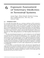
Figure 6.1 Spring densities of the winged form of the aphid, Aphis fabae, in large part reflect their carriage on the wind. (a) A. fabae eggs
are found on spindle plants and their distribution in the UK over winter reflects that of the plants (log
10
geometric mean number of eggs
per 100 spindle buds). (b) But by spring, although the highest densities are in spindle regions, the aphids have dispersed on the wind over
the whole country (log
10
geometric mean aerial density). (After Compton, 2001; from Cammell et al., 1989.)
EIPC06 10/24/05 1:55 PM Page 164
DISPERSAL, DORMANCY AND METAPOPULATIONS 165
floor have spines or prickles that increase their chance of being
carried passively on the coats of animals. The seeds may then be
concentrated in nests or burrows when the animal grooms itself.
The fruits of many shrubs and lower canopy trees are fleshy and
attractive to birds, and the seed coats resist digestion in the gut.
Where the seed is dispersed to is then somewhat less certain,

depending on the defecating behavior of the bird. It is usually
presumed that such associations are ‘mutualistic’ (beneficial to
both parties – see Chaper 13): the seed is dispersed in a more or
less predictable fashion; the disperser consumes either the fleshy
‘reward’ or a proportion of the seeds (those that it finds again).
There are also important examples in which animals are dis-
persed by an active agent. For instance, there are many species
of mite that are taken very effectively and directly from dung
pat to dung pat, or from one piece of carrion to another, by
attaching themselves to dung or carrion beetles. They usually attach
to a newly emerging adult, and leave again when that adult reaches
a new patch of dung or carrion. This, too, is typically mutualis-
tic: the mites gain a dispersive agent, and many of them attack
and eat the eggs of flies that would otherwise compete with the
beetles.
6.2.3 Active discovery and exploration
Many other animals cannot be said to explore, but they certainly
control their settlement (‘stopping’, see Section 6.1.1) and cease
movement only when an acceptable site has been found. For
example, most aphids, even in their winged form, have powers
of flight that are too weak to counteract the forces of prevailing
winds. But they control their take-off from their site of origin,
they control when they drop out of the windstream, and they
make additional, often small-scale flights if their original site
of settlement is unsatisfactory. In a precisely analogous manner,
the larvae of many river invertebrates make use of the flowing
column of water for dispersing from hatching sites to appropri-
ate microhabitats (‘invertebrate drift’) (Brittain & Eikeland, 1988).
The dispersal of aphids in the wind and of drifting invertebrates
in streams, therefore, involves ‘discovery’, over which they have

some, albeit limited, control.
Other animals explore, visiting many sites before returning to
a favored suitable one. For example, in contrast to their drifting
larvae, most adults of freshwater insects depend on flight for
upstream dispersal and movement from stream to stream. They
••••
% of density at edge of source area
25001000500
0
0
1
10
100
Distance (m)
(b)
1500 2000
Seeds per m
2
1206020
0
0
10
20
30
40
Distance (m)
(a)
5
15
25

80 100
Fraxinus
Lonchocarpus
Platypodium
Betula
Pinus
Tilia
Figure 6.2 (a) The density of wind-
dispersed seeds from solitary trees within
forests. The studies had a reasonable
density of sampling points, there were no
nearby conspecific trees and the source tree
was neither in a clearing nor at the forest
edge. (b) Observed long-distance dispersal
up to 1.6 km of wind dispersed seeds from
a forested source area. (After Greene &
Calogeropoulos, 2001, where the original
data sources may also be found.)
EIPC06 10/24/05 1:55 PM Page 165
166 CHAPTER 6
explore and, if successful, discover, suitable sites within which to
lay their eggs: starting, moving and stopping are all under active
control.
6.2.4 Clonal dispersal
In almost all modular organisms (see Section 4.2.1), an individual
genet branches and spreads its parts around it as it grows. There
is a sense, therefore, in which a developing tree or coral actively
disperses its modules into, and explores, the surrounding environ-
ment. The interconnections of such a clone often decay, so that
it becomes represented by a number of dispersed parts. This may

result ultimately in the product of one zygote being represented
by a clone of great age that is spread over great distances. Some
clones of the rhizomatous bracken fern (Pteridium aquilinum)
were estimated to be more than 1400 years old and one extended
over an area of nearly 14 ha (Oinonen, 1967).
We can recognize two extremes in
a continuum of strategies in clonal dis-
persal (Lovett Doust & Lovett Doust,
1982; Sackville Hamilton et al., 1987). At
one extreme, the connections between modules are long and the
modules themselves are widely spaced. These have been called
‘guerrilla’ forms, because they give the plant, hydroid or coral a
character like that of a guerrilla army. Fugitive and opportunist,
they are constantly on the move, disappearing from some ter-
ritories and penetrating into others. At the other extreme are
‘phalanx’ forms, named by analogy with the phalanxes of a Roman
army, tightly packed with their shields held around them. Here,
the connections are short and the modules are tightly packed, and
the organisms expand their clones slowly, retain their original
site occupancy for long periods, and neither penetrate readily
amongst neighboring plants nor are easily penetrated by them.
Even amongst trees, it is easy to see that the way in which
the buds are placed gives them a guerrilla or a phalanx type of
growth form. The dense packing of shoot modules in species
like cypresses (Cupressus) produces a relatively undispersed and
impenetrable phalanx canopy, whilst many loose-structured,
broad-leaved trees (Acacia, Betula) can be seen as guerrilla canopies,
bearing buds that are widely dispersed and shoots that interweave
with the buds and branches of neighbors. The twining or clam-
bering lianas in a forest are guerrilla growth forms par excellence,

dispersing their foliage and buds over immense distances, both
vertically and laterally.
The way in which modular organisms disperse and display their
modules affects the ways in which they interact with their neigh-
bors. Those with a guerrilla form will continually meet and com-
pete with other species and other genets of their own kind. With
a phalanx structure, however, most meetings will be between
modules of a single genet. For a tussock grass or a cypress tree,
competition must occur very largely between parts of itself.
Clonal growth is most effective as a means of dispersal in aquatic
environments. Many aquatic plants fragment easily, and the parts
of a single clone become independently dispersed because they
are not dependent on the presence of roots to maintain their
water relations. The major aquatic weed problems of the world
are caused by plants that multiply as clones and fragment and
fall to pieces as they grow: duckweeds (Lemna spp.), the water
hyacinth (Eichhornia crassipes), Canadian pond weed (Elodea
Canadensis) and the water fern Salvinia.
6.3 Patterns of distribution: dispersion
The movements of organisms affect the spatial pattern of their
distribution (their dispersion) and we can recognize three main pat-
terns of dispersion, although they too form part of a continuum
(Figure 6.3).
Random dispersion occurs when
there is an equal probability of an
organism occupying any point in space
(irrespective of the position of any
others). The result is that individuals are unevenly distributed
because of chance events.
Regular dispersion (also called a uniform or even distribution or

overdispersion) occurs either when an individual has a tendency to
avoid other individuals, or when individuals that are especially
close to others die. The result is that individuals are more evenly
spaced than expected by chance.
Aggregated dispersion (also called a contagious or clumped dis-
tribution or underdispersion) occurs either when individuals tend
to be attracted to (or are more likely to survive in) particular parts
of the environment, or when the presence of one individual
••••
AggregatedRegularRandom
Figure 6.3 Three generalized spatial patterns that may be
exhibited by organisms across their habitats.
guerrillas and
phalanx-formers
random, regular
and aggregated
distributions
EIPC06 10/24/05 1:55 PM Page 166
DISPERSAL, DORMANCY AND METAPOPULATIONS 167
attracts, or gives rise to, another close to it. The result is that
individuals are closer together than expected by chance.
How these patterns appear to an observer, however, and their
relevance to the life of other organisms, depends on the spatial
scale at which they are viewed. Consider the distribution of an
aphid living on a particular species of tree in a woodland. At a
large scale, the aphids will appear to be aggregated in particular
parts of the world, i.e. in woodlands as opposed to other types
of habitat. If samples are smaller and taken only in woodlands,
the aphids will still appear to be aggregated, but now on their
host tree species rather than on trees in general. However, if

samples are smaller still (25 cm
2
, about the size of a leaf ) and are
taken within the canopy of a single tree, the aphids might appear
to be randomly distributed over the tree as a whole. At an even
smaller scale (c. 1 cm
2
) we might detect a regular distribution
because individual aphids on a leaf avoid one another.
6.3.1 Patchiness
In practice, the populations of all spe-
cies are patchily distributed at some
scale or another, but it is crucial to
describe dispersion at scales that are
relevant to the lifestyle of the organisms concerned. MacArthur
and Levins (1964) introduced the concept of environmental grain
to make this point. For example, the canopy of an oak–hickory
forest, from the point of view of a bird like the scarlet tanager
(Piranga olivacea) that forages indiscriminately in both oaks and
hickories, is fine grained: i.e. it is patchy, but the birds experience
the habitat as an oak–hickory mixture. The habitat is coarse
grained, however, for defoliating insects that attack either oaks or
hickories preferentially: they experience the habitat one patch at
a time, moving from one preferred patch to another (Figure 6.4).
Patchiness may be a feature of the physical environment:
islands surrounded by water, rocky outcrops in a moorland, and
so on. Equally important, patchiness may be created by the
activities of organisms themselves; by their grazing, the deposi-
tion of dung, trampling or by the local depletion of water and
mineral resources. Patches in the environment that are created

by the activity of organisms have life histories. A gap created in
a forest by a falling tree is colonized and grows up to contain mature
trees, whilst other trees fall and create new gaps. The dead leaf
in a grassland area is a patch for colonization by a succession of
fungi and bacteria that eventually exhaust it as a resource, but
new dead leaves arise and are colonized elsewhere.
Patchiness, dispersal and scale are tied intimately together.
A framework that is useful in thinking about this distinguishes
between local and landscape scales (though what is ‘local’ to a
worm is very different from what is local to the bird that eats it)
and between turnover and invasion dispersal (Bullock et al., 2002).
Turnover dispersal at the local scale describes the movement into
a gap from occupied habitat immediately surrounding the gap;
whereas that gap may also be invaded or colonized by individuals
moving in from elsewhere in the surrounding community. At the
landscape scale, similarly, dispersal may be part of an on-going
turnover of extinction and recolonization of occupiable patches
within an otherwise unsuitable habitat matrix (e.g. islands in a
stream: ‘metapopulation dynamics’ – see Section 6.9, below), or
dispersal may result in the invasion of habitat by a ‘new’ species
expanding its range.
6.3.2 Forces favoring aggregations (in space and time)
The simplest evolutionary explanation for the patchiness of popu-
lations is that organisms aggregate when and where they find
resources and conditions that favor reproduction and survival.
These resources and conditions are usually patchily distributed
in both space and time. It pays (and has paid in evolutionary time)
••••
(a)
(Time 1 and time

2 and time 3 )
(Time 1 and time
2 and time 3 )
(b)
Time 5
Time 4
Time 3
Time 1 Time 2
Figure 6.4 The ‘grain’ of the environment must be seen from
the perspective of the organism concerned. (a) An organism
that is small or moves little is likely to see the environment
as coarse-grained: it experiences only one habitat type within
the environment for long periods or perhaps all of its life.
(b) An organism that is larger or moves more may see the same
environment as fine-grained: it moves frequently between habitat
types and hence samples them in the proportion in which they
occur in the environment as a whole.
fine- and coarse-
grained environments
EIPC06 10/24/05 1:55 PM Page 167
168 CHAPTER 6
to disperse to these patches when and where they occur. There
are, however, other specific ways in which organisms may gain
from being close to neighbors in space and time.
An elegant theory identifying a
selective advantage to individuals that
aggregate with others was suggested
by Hamilton (1971) in his paper
‘Geometry for the selfish herd’. He argued that the risk to an
individual from a predator may be lessened if it places another

potential prey individual between itself and the predator. The
consequence of many individuals doing this is bound to be an
aggregation. The ‘domain of danger’ for individuals in a herd is
at the edge, so that an individual would gain an advantage if
its social status allowed it to assimilate into the center of a herd.
Subordinate individuals might then be forced into the regions of
greater danger on the edge of the flock. This seems to be the case
in reindeer (Rangifer tarandus) and woodpigeons (Columba palum-
bus), where a newcomer may have to join the herd or flock at its
risky perimeter and can only establish itself in a more protected
position within the flock after social interaction (Murton et al., 1966).
Individuals may also gain from living in groups if this helps to
locate food, give warning of predators or if it pays for individuals
to join forces in fighting off a predator (Pulliam & Caraco, 1984).
The principle of the selfish herd as described for the aggrega-
tion of organisms in space is just as appropriate for the synchronous
appearance of organisms in time. The individual that is precocious
or delayed in its appearance, outside the norm for its population,
may be at greater risk from predators than those conformist indi-
viduals that take part in ‘flooding the market’ thereby diluting their
own risk. Amongst the most remarkable examples of synchrony
are the ‘periodic cicadas’ (insects), the adults of which emerge simul-
taneously after 13 or 17 years of life underground as nymphs.
Williams et al. (1993) studied the mortality of populations of
13-year periodic cicadas that emerged in northwestern Arkansas
in 1985. Birds consumed almost all of the standing crop of
cicadas when the density was low, but only 15–40% when the
cicadas reached peak density. Predation then rose to near 100%
as the cicada density fell again (Figure 6.5). Equivalent arguments
apply to the many species of tree, especially in temperate regions,

that have synchronous ‘mast’ years (see Section 9.4).
6.3.3 Forces diluting aggregations: density-dependent
dispersal
There are also strong selective pressures that can act against
aggregation in space or time. In some species a group of individuals
may actually concentrate a predator’s attention (the opposite
effect to the ‘selfish herd’). However, the foremost diluting forces
are certain to be the more intense competition suffered by
crowded individuals (see Chapter 5) and the direct interference
between such individuals even in the absence of a shortage of
resources. One likely consequence is that the highest rates of
dispersal will be away from the most crowded patches: density-
dependent emigration dispersal (Figure 6.6) (Sutherland et al., 2002),
though as we shall see below, density-dependent dispersal is by
no means a general rule.
Overall, though, the types of distribution over available
patches found in nature are bound to be compromises between
forces attracting individuals to disperse towards one another and
forces provoking individuals to disperse away from one another.
As we shall see in a later chapter, such compromises are con-
ventionally crystallized in the ‘ideal free’ and other theoretical
distributions (see Section 9.6.3).
6.4 Patterns of migration
6.4.1 Tidal, diurnal and seasonal movements
Individuals of many species move en masse from one habitat
to another and back again repeatedly during their life. The
timescale involved may be hours, days, months or years. In
some cases, these movements have the effect of maintaining the
••••
aggregation and

the selfish herd
Numbers (10
3
m
–2
)
0
2000
4000
6000
Predation (%)
0
20
40
100
60
80
Standing crop
Predation (%)
6249 29
May June
Figure 6.5 Changes in the density of a
population of 13-year periodical cicadas
in northwestern Arkansas in 1985, and
changes in the percentage eaten by birds.
(After Williams et al., 1993.)
EIPC06 10/24/05 1:55 PM Page 168
DISPERSAL, DORMANCY AND METAPOPULATIONS 169
organism in the same type of environment. This is the case in
the movement of crabs on a shoreline: they move with the

advance and retreat of the tide. In other cases, diurnal migration
may involve moving between two environments: the funda-
mental niches of these species can only be satisfied by alternat-
ing life in two distinct habitats within each day of their lives. For
example, some planktonic algae both in the sea and in lakes descend
to the depths at night but move to the surface during the day.
They accumulate phosphorus and perhaps other nutrients in the
deeper water at night before returning to photosynthesize near
the surface during daylight hours (Salonen et al., 1984). Other species
aggregate into tight populations during a resting period and
separate from each other when feeding. For example, most land
snails rest in confined humid microhabitats by day, but range widely
when they search for food by night.
Many organisms make seasonal migrations – again, either
tracking a favorable habitat or benefitting from different,
complementary habitats. The altitudinal migration of grazing ani-
mals in mountainous regions is one example. The American elk
(Cervus elaphus) and mule deer (Odocoileus hemionus), for instance,
move up into high mountain areas in the summer and down to
the valleys in the winter. By migrating seasonally the animals escape
the major changes in food supply and climate that they would
meet if they stayed in the same place. This can be contrasted with
the ‘migration’ of amphibians (frogs, toads, newts) between an
aquatic breeding habitat in spring and a terrestrial environment
for the remainder of the year. The young develop (as tadpoles)
in water with a different food resource from that which they will
later eat on land. They will return to the same aquatic habitat
for mating, aggregate into dense populations for a time and then
separate to lead more isolated lives on land.
6.4.2 Long-distance migration

The most remarkable habitat shifts are
those that involve traveling very long
distances. Many terrestrial birds in the northern hemisphere
move north in the spring when food supplies become abundant
during the warm summer period, and move south to savannas
in the fall when food becomes abundant only after the rainy
season. Both are areas in which seasons of comparative glut and
famine alternate. Migrants then make a large contribution to the
diversity of a local fauna. Of the 589 species of birds (excluding
seabirds) that breed in the Palaearctic (temperate Europe and Asia),
40% spend the winter elsewhere (Moreau, 1952). Of those species
that leave for the winter, 98% travel south to Africa. On an even
larger scale, the Arctic tern (Sterna paradisaea) travels from its Arctic
breeding ground to the Antarctic pack ice and back each year –
about 10,000 miles (16,100 km) each way (although unlike many
other migrants it can feed on its journey).
The same species may behave in different ways in different
places. All robins (Erithacus rubecula) leave Finland and Sweden
in winter, but on the Canary Islands the species is resident the
whole year-round. In most of the intervening countries, a part
of the population migrates and a part remains resident. Such
variations are in some cases associated with clear evolutionary
divergence. This is true of the knot (Calidris canutus), a species of
small wading bird mostly breeding in remote areas of the Arctic
tundras and ‘wintering’ in the summers of the southern hemisphere.
At least five subspecies appear to have diverged in the Late
Pleistocene (based on genetic evidence from the sequencing of
mitochondrial DNA), and these now have strikingly different
patterns of distribution and migration (Figure 6.7).
••••

0
0
1
Number of larvae per mm
2
168
.5
(a)
0
0
75
Number of pairs
20001000
50
(b)
Emigration Observed dispersal
Natal dispersal (%)
Dispersal rate (log scale)
25
Figure 6.6 Density-dependent dispersal. (a) The dispersal rates of newly hatched blackfly (Simulium vittatum) larvae increase with
increasing density. (Data from Fonseca & Hart, 1996.) (b) The percentage of juvenile male barnacle geese, Branta leucopsis, dispersing
from breeding colonies on islands in the Baltic Sea to non-natal breeding locations increased as density increased. (Data from van der
Juegd 1999.) (After Sutherland et al., 2002.)
birds
EIPC06 10/24/05 1:55 PM Page 169
170 CHAPTER 6
Long-distance migration is a feature of many other groups too.
Baleen whales in the southern hemisphere move south in sum-
mer to feed in the food-rich waters of the Antarctic. In winter
they move north to breed (but scarcely to feed) in tropical and

subtropical waters. Caribou (Rangifer tarandus) travel several
hundred kilometers per year from northern forests to the tundra
and back. In all of these examples, an individual of the migrating
species may make the return journey several times.
Many long-distance migrants, how-
ever, make only one return journey
during their lifetime. They are born in
one habitat, make their major growth in another habitat, but
then return to breed and die in the home of their infancy. Eels
and migratory salmon provide classic examples. The European
eel (Anguilla anguilla) travels from European rivers, ponds and lakes
across the Atlantic to the Sargasso Sea, where it is thought to repro-
duce and die (although spawning adults and eggs have never actu-
ally been caught there). The American eel (Anguilla rostrata) makes
a comparable journey from areas ranging between the Guianas
in the south, to southwest Greenland in the north. Salmon make
a comparable transition, but from a freshwater egg and juvenile
phase to mature as a marine adult. The fish then returns to
freshwater sites to lay eggs. After spawning, all Pacific salmon
(Oncorhynchus nerka) die without ever returning to the sea. Many
Atlantic salmon (Salmo salar) also die after spawning, but some
survive to return to the sea and then migrate back upstream to
spawn again.
6.4.3 ‘One-way only’ migration
In some migratory species, the journey for an individual is on a
strictly one-way ticket. In Europe, the clouded yellow (Colias croceus),
red admiral (Vanessa atalanta) and painted lady (Vanessa cardui)
butterflies breed at both ends of their migrations. The individuals
that reach Great Britain in the summer breed there, and their off-
spring fly south in autumn and breed in the Mediterranean region

– the offspring of these in turn come north in the following summer.
Most migrations occur seasonally in the life of individuals
or of populations. They usually seem to be triggered by some
••••
Breeding area
Staging area
Wintering area
Staging and wintering area
Migratory corridors
180°
0°
140°
30°
45°
100°
60°
20°
20°
20°
30°
60°
100°
140°
180°
160°
30°
45°
0°
30°
75°

60°
roselaari
rogersi
canutus
rufa
islandica
islandica
canutus
Figure 6.7 Global distribution and migration pattern of knots (Calidris spp.). Solid shading indicates the breeding areas; horizontally
striped spots indicate the stop-over areas, used only during south- and northward migration; the cross-hatched spots indicate the areas
used both as stop-over and wintering sites; and the vertically striped spots designate areas used only for wintering. The gray shaded
corridors indicate proven migration routes; the broken-shaded corridors indicate tentative migration routes suggested in the literature.
(After Piersma & Davidson, 1992.)
eels and salmon
EIPC06 10/24/05 1:55 PM Page 170
DISPERSAL, DORMANCY AND METAPOPULATIONS 171
external seasonal phenomenon (e.g. changing day length), and
sometimes also by an internal physiological clock. They are often
preceded by quite profound physiological changes such as the
accumulation of body fat. They represent strategies evolved in
environments where seasonal events like rainfall and temperature
cycles are reliably repeated from year to year. There is, however,
a type of migration that is tactical, forced by events such as over-
crowding, and appears to have no cycle or regularity. These are
most common in environments where rainfall is not seasonally
reliable. The economically disastrous migration plagues of locusts
in arid and semiarid regions are the most striking examples.
6.5 Dormancy: migration in time
An organism gains in fitness by dispersing its progeny as long
as the progeny are more likely to leave descendants than if they

remained undispersed. Similarly, an organism gains in fitness by
delaying its arrival on the scene, so long as the delay increases its
chances of leaving descendants. This will often be the case when
conditions in the future are likely to be better than those in the
present. Thus, a delay in the recruitment of an individual to a
population may be regarded as ‘migration in time’.
Organisms generally spend their period of delay in a state of
dormancy. This relatively inactive state has the benefit of conserving
energy, which can then be used during the period following the
delay. In addition, the dormant phase of an organism is often more
tolerant of the adverse environmental conditions prevailing dur-
ing the delay (i.e. tolerant of drought, extremes of temperature,
lack of light and so on). Dormancy can be either predictive or
consequential (Müller, 1970). Predictive dormancy is initiated in
advance of the adverse conditions, and is most often found in
predictable, seasonal environments. It is generally referred to as
‘diapause’ in animals, and in plants as ‘innate’ or ‘primary’ dormancy
(Harper, 1977). Consequential (or ‘secondary’) dormancy, on
the other hand, is initiated in response to the adverse conditions
themselves.
6.5.1 Dormancy in animals: diapause
Diapause has been most intensively studied in insects, where
examples occur in all developmental stages. The common field
grasshopper Chorthippus brunneus is a fairly typical example. This
annual species passes through an obligatory diapause in its egg stage,
where, in a state of arrested development, it is resistant to the
cold winter conditions that would quickly kill the nymphs and
adults. In fact, the eggs require a long cold period before develop-
ment can start again (around 5 weeks at 0°C, or rather longer at
a slightly higher temperature) (Richards & Waloff, 1954). This

ensures that the eggs are not affected by a short, freak period
of warm winter weather that might then be followed by normal,
dangerous, cold conditions. It also means that there is an
enhanced synchronization of subsequent development in the
population as a whole. The grasshoppers ‘migrate in time’ from
late summer to the following spring.
Diapause is also common in species
with more than one generation per
year. For instance, the fruit-fly Droso-
phila obscura passes through four generations per year in
England, but enters diapause during only one of them (Begon,
1976). This facultative diapause shares important features with
obligatory diapause: it enhances survivorship during a predictably
adverse winter period, and it is experienced by resistant diapause
adults with arrested gonadal development and large reserves
of stored abdominal fat. In this case, synchronization is achieved
not only during diapause but also prior to it. Emerging adults
react to the short daylengths of the fall by laying down fat and
entering the diapause state; they recommence development in
response to the longer days of spring. Thus, by relying, like many
species, on the utterly predictable photoperiod as a cue for seasonal
development, D. obscura enters a state of predictive diapause that
is confined to those generations that inevitably pass through the
adverse conditions.
Consequential dormancy may be expected to evolve in envir-
onments that are relatively unpredictable. In such circumstances,
there will be a disadvantage in responding to adverse conditions
only after they have appeared, but this may be outweighed by
the advantages of: (i) responding to favorable conditions immedi-
ately after they reappear; and (ii) entering a dormant state only if

adverse conditions do appear. Thus, when many mammals enter
hibernation, they do so (after an obligatory preparatory phase)
in direct response to the adverse conditions. Having achieved ‘resist-
ance’ by virtue of the energy they conserve at a lowered body
temperature, and having periodically emerged and monitored their
environment, they eventually cease hibernation whenever the
adversity disappears.
6.5.2 Dormancy in plants
Seed dormancy is an extremely widespread phenomenon in
flowering plants. The young embryo ceases development whilst
still attached to the mother plant and enters a phase of suspended
activity, usually losing much of its water and becoming dormant
in a desiccated condition. In a few species of higher plants, such
as some mangroves, a dormant period is absent, but this is very
much the exception – almost all seeds are dormant when they
are shed from the parent and require special stimuli to return them
to an active state (germination).
Dormancy in plants, though, is not confined to seeds. For
example, as the sand sedge Carex arenaria grows, it tends to
accumulate dormant buds along the length of its predominantly
linear rhizome. These may remain alive but dormant long after
••••
the importance of
photoperiod
EIPC06 10/24/05 1:55 PM Page 171
172 CHAPTER 6
the shoots with which they were produced have died, and they
have been found in numbers of up to 400–500 m
−2
(Noble et al.,

1979). They play a role analogous to the bank of dormant seeds
produced by other species.
Indeed, the very widespread habit of deciduousness is a form
of dormancy displayed by many perennial trees and shrubs.
Established individuals pass through periods, usually of low
temperatures and low light levels, in a leafless state of low
metabolic activity.
Three types of dormancy have
been distinguished.
1 Innate dormancy is a state in which there is an absolute
requirement for some special external stimulus to reactivate
the process of growth and development. The stimulus may
be the presence of water, low temperature, light, photoperiod
or an appropriate balance of near- and far-red radiation.
Seedlings of such species tend to appear in sudden flushes
of almost simultaneous germination. Deciduousness is also an
example of innate dormancy.
2 Enforced dormancy is a state imposed by external conditions
(i.e. it is consequential dormancy). For example, the Missouri
goldenrod Solidago missouriensis enters a dormant state when
attacked by the beetle Trirhabda canadensis. Eight clones,
identified by genetic markers, were followed prior to, during
and after a period of severe defoliation. The clones, which
varied in extent from 60 to 350 m
2
and from 700 to 20,000
rhizomes, failed to produce any above-ground growth (i.e.
they were dormant) in the season following defoliation and
had apparently died, but they reappeared 1–10 years after they
had disappeared, and six of the eight bounced back strongly

within a single season (Figure 6.8). Generally, the progeny
of a single plant with enforced dormancy may be dispersed
in time over years, decades or even centuries. Seeds of
Chenopodium album collected from archeological excavations have
been shown to be viable when 1700 years old (Ødum, 1965).
3 Induced dormancy is a state produced in a seed during a period
of enforced dormancy in which it acquires some new require-
ment before it can germinate. The seeds of many agricultural
and horticultural weeds will germinate without a light stim-
ulus when they are released from the parent; but after a
period of enforced dormancy they require exposure to light
before they will germinate. For a long time it was a puzzle
that soil samples taken from the field to the laboratory would
quickly generate huge crops of seedlings, although these same
seeds had failed to germinate in the field. It was a simple idea
of genius that prompted Wesson and Wareing (1969) to col-
lect soil samples from the field at night and bring them to the
laboratory in darkness. They obtained large crops of seedlings
from the soil only when the samples were exposed to light.
This type of induced dormancy is responsible for the accu-
mulation of large populations of seeds in the soil. In nature
they germinate only when they are brought to the soil
surface by earthworms or other burrowing animals, or by the
exposure of soil after a tree falls.
Seed dormancy may be induced by radiation that contains a
relatively high ratio of far-red (730 nm) to near-red (approx-
imately 660 nm) wavelengths, a spectral composition character-
istic of light that has filtered through a leafy canopy. In nature,
this must have the effect of holding sensitive seeds in the
dormant state when they land on the ground under a canopy,

whilst releasing them into germination only when the over-
topping plants have died away.
Most of the species of plants with seeds that persist for long
in the soil are annuals and biennials, and they are mainly weedy
species – opportunists waiting (literally) for an opening. They largely
lack features that will disperse them extensively in space. The seeds
of trees, by contrast, usually have a very short expectation of life
in the soil, and many are extremely difficult to store artificially for
more than 1 year. The seeds of many tropical trees are particu-
larly short lived: a matter of weeks or even days. Amongst trees,
••••
innate, enforced and
induced dormancy
(a)
Period 1 Period 2
Defoliated clone territory recovered (%)
1990 1995 2000
60m
2
15,000
(b)
150m
2
7500
(c)
350m
2
20,000
(d)
170m

2
3000
(e)
40m
2
3700
(f)
150m
2
12,000
(g)
150m
2
12,000
(h)
150m
2
12,000
100
0
100
0
100
0
100
0
100
0
100
0

100
0
100
0
Year
Figure 6.8 The histories of eight Missouri goldenrod (Solidago
missouriensis) clones (rows a–h). Each clone’s predefoliation
area (m
2
) and estimated number of ramets is given on the left.
The panels show a 15-year record of the presence (shading) and
absence of ramets in each clone’s territory. The arrowheads show
the beginning of dormancy, initiated by a Trirhabda canadensis
eruption and defoliation. Reoccupation of entire or major
segments of the original clone’s territory by postdormancy ramets
is expressed as the percentage of the original clone’s territory.
(After Morrow & Olfelt, 2003.)
EIPC06 10/24/05 1:55 PM Page 172
DISPERSAL, DORMANCY AND METAPOPULATIONS 173
the most striking longevity is seen in those that retain the seeds
in cones or pods on the tree until they are released after fire (many
species of Eucalyptus and Pinus). This phenomenon of serotiny pro-
tects the seeds against risks on the ground until fire creates an
environment suitable for their rapid establishment.
6.6 Dispersal and density
Density-dependent emigration was identified in Section 6.3.3 as
a frequent response to overcrowding. We turn now to the more
general issue of the density dependence of dispersal and also to
the evolutionary forces that may have led to any density depen-
dences that are apparent. In doing so, it is important to bear in

mind the point made earlier (see Section 6.1.1): that ‘effective’ dis-
persal (from one place to another) requires emigration, transfer
and immigration. The density dependences of the three need not
be the same.
6.6.1 Inbreeding and outbreeding
Much of this chapter is devoted to the demographic or ecological
consequences of dispersal, but there are also important genetic
and evolutionary consequences. Any evolutionary ‘consequence’
is, of course, then a potentially important selective force favor-
ing particular patterns of dispersal or indeed the tendency to dis-
perse at all. In particular, when closely related individuals breed,
their offspring are likely to suffer an ‘inbreeding depression’
in fitness (Charlesworth & Charlesworth, 1987), especially as a
result of the expression in the phenotype of recessive deleterious
alleles. With limited dispersal, inbreeding becomes more likely,
and inbreeding avoidance is thus a force favoring dispersal. On
the other hand, many species show local adaptation to their
immediate environment (see Section 1.2). Longer distance dispersal
may therefore bring together genotypes adapted to different
local environments, which on mating give rise to low-fitness
offspring adapted to neither habitat. This is called ‘outbreeding
depression’, resulting from the break-up of coadapted combina-
tions of genes – a force acting against dispersal. The situation is
complicated by the fact that inbreeding depression is most likely
amongst populations that normally outbreed, since inbreeding itself
will purge populations of their deleterious recessives. None the
less, natural selection can be expected to favor a pattern of
dispersal that is in some sense intermediate – maximizing fitness
by avoiding both inbreeding and outbreeding depression, though
these will clearly be by no means the only selective forces acting

on dispersal.
Certainly, there are several examples in plants of inbreeding
and outbreeding depression when pollen is transferred from
either close or distant donors, and in some cases both effects
can be demonstrated in a single experiment. For example, when
larkspur (Delphinium nelsonii) offspring were generated by hand
pollinating with pollen brought from 1, 3, 10 and 30 m to the
receptor flowers (Figure 6.9), both inbreeding and outbreeding
depression in fitness were apparent.
6.6.2 Avoiding kin competition
In fact, inbreeding avoidance is not the only force likely to favor
natal dispersal of offspring away from their close relatives. Such
••••
Overall fitness
101
0.0
0.4
0.7
3
(c)
0.6
0.9
0.5
0.8
30
0.3
0.2
0.1
Progeny size in third year of life
101

0
10
40
70
3
Crossing distance (m)
(a)
30
60
20
50
30
Progeny lifespan (years)
101
0
2
5
3
(b)
1
4
3
30
Crossing distance (m) Crossing distance (m)
Figure 6.9 Inbreeding and outbreeding depression in Delphinium nelsonii: (a) progeny size in the third year of life, (b) progeny lifespan
and (c) the overall fitness of progeny cohorts were all lower when progeny were the result of crosses with pollen taken close to (1 m) or
far from (30 m) the receptor plant. Bars show standard errors. (After Waser & Price, 1994.)
EIPC06 10/24/05 1:55 PM Page 173
174 CHAPTER 6
dispersal will also be favored because it decreases the likelihood

of competitive effects being directed at close kin. This was
explained in a classic modeling paper by Hamilton and May
(1977; see also Gandon & Michalakis, 2001), who demonstrated
that even in very stable habitats, all organisms will be under
selective pressure to disperse some of their progeny. Imagine a
population in which the majority of organisms have a stay-at-home,
nondispersive genotype O, but in which a rare mutant genotype,
X, keeps some offspring at home but commits others to dis-
persal. The disperser X will suffer no competition in its own patch
from O-type individuals but will compete against O-type individuals
in their home patches. Disperser X will direct much of its com-
petitive effects at non-kin (with genotype O), while O directs all
of its competition at kin (also with genotype O). X will therefore
increase in frequency in the population. On the other hand, if
the majority of the population are type X, whilst O is the rare
mutant, O will still do worse than X, since O can never displace
any of the Xs from their patches but has itself to contend with
several or many dispersers in its own patch. Dispersal is there-
fore said to be an evolutionarily stable strategy (ESS) (Maynard
Smith, 1972; Parker, 1984). A population of nondispersers will
evolve towards the ubiquitous possession of a dispersive tendency;
but a population of dispersers will be under no selective pressure
to lose that tendency. Hence, the avoidance of both inbreeding
and kin competition seem likely to give rise to higher emigration
rates at higher densities, when these forces are most intense.
There is indeed evidence for kin competition playing a role
in driving offspring away from their natal habitat (Lambin et al.,
2001), but much of it is indirect. For example, in the California
mouse, Peromyscus californicus, mean dispersal distance increased
with increasing litter size in males and, in females, with increas-

ing numbers of sisters in the litter (Ribble, 1992). The more kin
a young individual was surrounded by, the further it dispersed.
Lambin et al. (2001) concluded in their review, though, that
whereas there is plentiful evidence for density-dependent emigration
(see Section 6.3.3), there is little evidence for density-dependent
‘effective’ dispersal (emigration, transfer and immigration), in
part at least because immigration (and perhaps transfer) may be
inhibited at high densities. For example, in a study of kangaroo
rats, Dipodomys spectabilis, over several years during which
density varied, dispersal was monitored first after juveniles had
become independent of their parents, but then again after they
had survived to breed themselves. The kangaroo rats occupy
complex burrow systems containing food reserves, and these
remain more or less constant in number: high densities therefore
mean a saturated environment and more intense competition
( Jones et al., 1988). At the time of juvenile independence, density
had no effect on dispersal (i.e. on emigration); but by first breed-
ing, dispersal rates (i.e. effective dispersal rates) were lower at
higher densities (inverse density dependence) (Figure 6.10). In males,
this was mainly because they moved less between juvenile inde-
pendence and breeding. In females, it occurred mainly because
their survival rate in new patches was lower at high densities
( Jones, 1988).
6.6.3 Philopatry
Effective dispersal is not straightforwardly density dependent at
least in part because there are also selective forces in favor of not
dispersing, but instead showing so-called philopatry or ‘home-
loving’ behavior (Lambin et al., 2001). This can come about
because there are advantages of inhabiting a familiar environment;
or individuals may cooperate with (or at least be prepared to

tolerate) related individuals in the natal habitat that share a high
proportion of their genes; or individuals that do disperse may be
confronted with a ‘social fence’ of aggression or intolerance from
groups of unrelated individuals (Hestbeck, 1982). These forces, too,
may become more intense as the environment becomes more
saturated. Thus, for example, Lambin and Krebs (1993) found in
Townsend’s voles, Microtus townsendii, in Canada, that the nests
or centers of activities of females that were first degree relatives
(mother–daughters, littermate sisters) were closer than those
that were second degree relatives (nonlittermate sisters, aunt–
nieces), which were closer than those that were more distantly
related, which in turn were closer than those not related at all.
••••
0
20
Dispersal distance
at first breeding (m)
10
Number of individuals
0
1–50
51–100
101–150
151–200
>200
(b)
0
20
10
Number of individuals

(a)
Low density
0
20
10
0
1–50
51–100
101–150
151–200
>200
0
20
10
High density
Figure 6.10 Inverse density-dependent effective dispersal in the
kangaroo rat, Dipodomys spectabilis: (a) males, (b) females. Natal
dispersal distances were greater at low than at high densities.
(After Jones, 1988.)
EIPC06 10/24/05 1:55 PM Page 174
DISPERSAL, DORMANCY AND METAPOPULATIONS 175
And in a study of Belding’s ground squirrels, Spermophilus beldingi,
even when females dispersed, they tended to settle near their
sisters (Nunes et al., 1997). Moreover, there are examples of fit-
ness being higher when close kin are nearby. For instance, Lambin
and Yoccoz (1998) manipulated the relatedness of groups of
breeding females of Townsend’s vole, mimicking either a situa-
tion where the population had experienced philopatric recruitment
followed by high survival (‘high kinship’), or where the popula-
tion had experienced either low philopatric recruitment or high

mortality of recruits (‘low kinship’). Survival of pups, especially
early in their life, was significantly higher in the high kinship than
in the low kinship treatment.
Overall, then, the relationship between dispersal and density
will depend, just like all other adaptations, on evolved comprom-
ises to conflicting forces, and also on which aspect of dispersal
(emigration, effective dispersal, etc.) is the focus of attention. It
is no surprise either that, as we shall see below, the balance of
advantage works out differently for different groups: males and
females, old and young, and so on. Such variation also argues
against broad generalizations suggesting that dispersal is ‘typically’
at presaturation densities (i.e. before resource limitation is intense)
or for that matter at saturation densities (Lidicker, 1975).
6.7 Variation in dispersal within populations
6.7.1 Dispersal polymorphism
One source of variability in dispersal within populations is a
somatic polymorphism amongst the progeny of a single parent.
This is typically associated with habitats that are variable or
unpredictable. A classic example is the desert annual plant
Gymnarrhena micrantha. This bears very few (one to three) large
seeds (achenes) in flowers that remain unopened below the
soil surface, and these seeds germinate in the original site of the
parent. The root system of the seedling may even grow down
through the dead parent’s root channel. But the same plants also
produce above-ground, smaller seeds with a feathery pappus, and
these are wind dispersed. In very dry years only the undispersed
underground seeds are produced, but in wetter years the plants
grow vigorously and produce a large number of seeds above
ground, which are released to the haz-
ards of dispersal (Koller & Roth, 1964).

There are very many examples of
such seed dimorphism amongst the
flowering plants. Both the dispersed and the ‘stay at home’ seeds
will, in their turn, produce both dispersed and ‘stay at home’
progeny. Moreover, the ‘stay at home’ seed is often produced from
self-pollinated flowers below ground or from unopened flowers,
whereas the seeds that are dispersed are more often the product
of cross-fertilization. Hence, the tendency to disperse is coupled
with the possession of new, recombinant (‘experimental’) geno-
types, whereas the ‘stay at home’ progeny are more likely to be
the product of self-fertilization.
A dimorphism of dispersers and nondispersers is also a common
phenomenon amongst aphids (winged and wingless progeny). As
this differentiation occurs during the phase of population growth
when reproduction is parthenogenetic, the winged and wingless
forms are genetically identical. The winged morphs are clearly
more capable of dispersing to new habitats, but they also often
have longer development times, lower fecundity, shorter lifespans
and hence a reduced intrinsic rate of increase (Dixon, 1998). It is
perhaps no surprise, therefore, that aphids may modify the pro-
portions of winged and wingless morphs in immediate response
to the environments in which they find themselves. The pea aphid,
Acyrthosiphon pisum, for example, produces more winged morphs
in the presence of predators (Figure 6.11), presumably as an escape
response from an adverse environment.
••••
0
80
Period 1
20

% of winged offspring
(a)
70
60
50
40
30
10
Period 2
0
80
Period 1
20
(b)
70
60
50
40
30
10
Period 2
dispersal
dimorphisms
Figure 6.11 The mean proportion
(± SE) of winged morphs of the pea aphid,
Acyrthosiphon pisum, produced after two
separate periods of exposure to each of
two predators: (a) hoverfly larvae and
(b) lacewing larvae. Dark bars, predator
treatment; light bars, control. (After Kunert

& Weisser, 2003.)
EIPC06 10/24/05 1:55 PM Page 175
176 CHAPTER 6
6.7.2 Sex-related differences
Males and females often differ in their liability to disperse.
Differences are especially strong in some insects, where it is the
male that is usually the more active disperser. For example, in
the winter moth (Operophtera brumata), the female is wingless whilst
the male is free-flying. In a seminal paper, Greenwood (1980) con-
trasted the sex-biased dispersal of birds and mammals. Amongst
birds it is usually the females that are the main dispersers, but
amongst mammals it is usually the males. Evolutionary explana-
tions for a sex bias have emphasized on the one hand the advant-
ages of a sex bias in its own right as a means of minimizing
inbreeding, but also that details of the mating system may gen-
erate asymmetries in the costs and benefits of dispersal and
philopatry in the two sexes (Lambin et al., 2001). Thus, in birds,
competition for territories is typically most intense amongst
males. They, therefore, have most to gain from philopatry in terms
of being familiar with their natal habitat, whereas the dispersing
(and often monogamous) females may gain from exercising a
choice of mate amongst the males. In mammals, the (often
polygamous) males may compete more often for mates than for
territories, and they therefore have most to gain by dispersing to
areas with the largest number of defensible females.
6.7.3 Age-related differences
Much dispersal is natal dispersal, i.e. dispersal by juveniles before
they reproduce for the first time. In many taxa this is constitu-
tional: we have already noted that seed dispersal in plants is, by
its nature, natal dispersal. Likewise, many marine invertebrates

have a sessile adult (reproductive) stage and rely on their larvae
(obviously pre-reproductive) for dispersal. On the other hand,
most insects have a sessile larval stage and rely on the reproductive
adults for dispersal. Here, for iteroparous species, dispersal is most
often something that occurs throughout the adult life, before
and after the first breeding episode; but for semelparous species,
dispersal once again is almost inevitably natal.
Birds and mammals, once they have fledged or been weaned
and are independent of their mothers, also have the potential to
disperse throughout the rest of their lives. None the less, most
dispersal here, too, is natal (Wolff, 1997). Indeed, age-biases
and sex-biases in dispersal, and the forces of inbreeding-avoidance,
competition-avoidance and philopatry, are all tied intimately
together in the patterns of dispersal observed in mammals. Thus,
for example, in an experiment with gray-tailed voles, Microtus
canicaudus, 87% of juvenile males and 34% of juvenile females
dispersed within 4 weeks of initial capture at low densities, but
only 16% and 12%, respectively, dispersed at high densities (Wolff
et al., 1997). There was massive juvenile dispersal, which was
particularly pronounced in the males; and the inverse density
dependence, and especially the very high rates at low densities,
argue in favor of inbreeding-avoidance as a major force shaping
the pattern.
6.8 The demographic significance of dispersal
The ecological fact of life identified in Section 4.1 emphasized
that dispersal can have a potentially profound effect on the
dynamics of populations. In practice, however, many studies
have paid little attention to dispersal. The reason often given is
that emigration and immigration are approximately equal, and
they therefore cancel one another out. One suspects, though, that

the real reason is that dispersal is usually extremely difficult
to quantify.
The nature of the role of dispersal
in population dynamics depends on
how we think of populations. The
simplest view sees a population as a
collection of individuals distributed more or less continuously over
a stretch of more or less suitable habitat, such that the popula-
tion is a single, undivided entity. Dispersal is then a process
contributing to either the increase (immigration) or decrease
(emigration) in the population. Many populations, however, are
in fact metapopulations; that is, collections of subpopulations.
We noted in Section 6.3.1 the ubiquity of patchiness in eco-
logy and the importance of dispersal in linking patches to one
another. A subpopulation, then, occupies a habitable patch in
the landscape, and it corresponds, in isolation, to the simple
view of a population described above. But the dynamics of the
metapopulation as a whole is determined in large part by the
rate of extinction of individual subpopulations, and the rate
of colonization – by dispersal – of habitable but uninhabited
patches. Note, however, that just because a species occupies
more than one habitable site, each of which supports a popula-
tion, this does not mean that those populations comprise a
metapopulation. As we shall discuss more fully below, ‘classic’
metapopulation status is conferred only when extinction and
recolonization play a major role in the overall dynamics.
6.8.1 Modeling dispersal: the distribution of patches
The ways in which dispersal intervenes in the dynamics of
populations can be envisaged, or indeed modeled mathematically,
in three different ways (see Kareiva, 1990; Keeling, 1999). The first

is an ‘island’ or ‘spatially implicit’ approach (Hanski & Simberloff,
1997; Hanski, 1999). Here, the key feature is that a proportion
of the individuals leave their home patches and enter a pool of
dispersers and are then redistributed amongst patches, usually at
random. Thus, these models do not place patches at any specific
spatial location. All patches may lose or gain individuals through
dispersal, but all are, in a sense, equally distant from all other
••••
metapopulations and
subpopulations
EIPC06 10/24/05 1:55 PM Page 176
DISPERSAL, DORMANCY AND METAPOPULATIONS 177
patches. Many metapopulation models, including the earliest
(Levins’ model, see below), come into this category, and despite
their simplicity (real patches do have a location in space) they have
provided important insights, in part because their simplicity
makes them easier to analyze.
In contrast, spatially explicit models acknowledge that the
distances between patches vary, as do therefore the chances of
them exchanging individuals through dispersal. The earliest such
models, developed in population genetics, were linear ‘stepping
stones’, where dispersal occurred only between adjacent patches
in the line (Kimura & Weiss, 1964). More recently, spatially
explicit approaches have often involved ‘lattice’ models in which
patches are arranged on a (usually) square grid, and patches
exchange dispersing individuals with ‘neighboring’ patches –
perhaps the four with which they share a side, or the eight
with which they make any contact at all, including the diagonals
(Keeling, 1999). Of course, despite being spatially explicit, such
models are still caricatures of patch arrangements in the real world.

They are none the less useful in highlighting new dynamic patterns
that appear as soon as space is incorporated explicitly: not only
spatial patterns (see, for example, Section 10.5.6), but also altered
temporal dynamics, including, for example, the increased prob-
ability of extinction of whole spatially explicit metapopulations
as habitat is destroyed (Figure 6.12). Further spatially explicit
models are also spatially ‘realistic’ (see Hanski, 1999) in that they
include information about the actual geometry of fragmented
landscapes. One of these, the ‘incidence function model’ (Hanski,
1994b), is utilized below (Section 6.9.4).
Finally, the third approach treats space not as patchy at all but
as continuous and homogeneous, and usually models dispersal as
part of a reaction–diffusion system, where the dynamics at any
given location in space are captured by the ‘reaction’, and dispersal
is added as separate ‘diffusion’ terms. The approach has been more
useful in other areas of biology (e.g. developmental biology)
than it has in ecology. None the less, the mathematical under-
standing of such systems is strong, and they are particularly
good at demonstrating how spatial variation (i.e. patchiness) can
be generated, internally, within an intrinsically homogeneous
system (Kareiva, 1990; Keeling, 1999).
6.8.2 Dispersal and the demography of single
populations
The studies that have looked carefully at dispersal have tended to
bear out its importance. In a long-term and intensive investiga-
tion of a population of great tits, Parus major, near Oxford, UK,
it was observed that 57% of breeding birds were immigrants rather
than born in the population (Greenwood et al., 1978). In a pop-
ulation of the Colorado potato beetle, Leptinotarsa decemlineata,
in Canada, the average emigration rate of newly emerged adults

was 97% (Harcourt, 1971). This makes the rapid spread of the
beetle in Europe in the middle of the last century easy to under-
stand (Figure 6.13).
A profound effect of dispersal on the dynamics of a popula-
tion was seen in a study of Cakile edentula, a summer annual plant
growing on the sand dunes of Martinique Bay, Nova Scotia. The
population was concentrated in the middle of the dunes, and
declined towards both the sea and the land. Only in the area
towards the sea, however, was seed production high enough and
mortality sufficiently low for the population to maintain itself year
after year. At the middle and landward sites, mortality exceeded
seed production. Hence, one might have expected the population
••••
0
0.0
0.8
Habitat destroyed (D)
1.00.4
0.4
Sites occupied (V *)
0.80.2 0.6
0.2
0.6
Figure 6.12 In a series of models, as an increasing fraction of
habitat is destroyed (left to right on the x-axis), the fraction of
available sites occupied (y-axis) declines until the whole population
is effectively extinct (no sites occupied). The diagonal dotted line
shows the relationship for a spatially implicit model in which all
sites are equally connected. The dots show output from a spatially
explicit lattice model: values are the means of five replicates

(the model is probabilistic: each run is slightly different). Three
examples of the lattice are shown below, with 0.05. 0.40 and 0.70
of the patches destroyed (black). With little habitat destruction
(towards the left), an explicit spatial structure makes negligible
difference as the remaining patches are well connected to other
patches. But with more habitat destruction, patches in the lattice
become increasingly isolated and unlikely to be recolonized, and
many more of them remain unoccupied than in the spatially
implicit model. (After Bascompte & Sole, 1996.)
EIPC06 10/24/05 1:55 PM Page 177
••
178 CHAPTER 6
to become extinct (Figure 6.14). But the distribution of Cakile did
not change over time. Instead, large numbers of seeds from the
seaward zone dispersed to the middle and landward zones.
Indeed, more seeds were dispersed into and germinated in these
two zones than were produced by the residents. The distribution
and abundance of Cakile were directly due to the dispersal of seeds
in the wind and the waves.
Probably the most fundamental consequence of dispersal for
the dynamics of single populations, though, is the regulatory effect
of density-dependent emigration (see Section 6.3.3). Locally, all
that was said in Chapter 5 regarding density-dependent mor-
tality applies equally to density-dependent emigration. Globally,
of course, the consequences of the two may be quite different.
Those that die are lost forever and from everywhere. With
emigration, one population’s loss may be another’s gain.
6.8.3 Invasion dynamics
In almost every aspect of life, there
is a danger in imagining that what is

usual and ‘normal’ is in fact universal,
and that what is unusual or eccentric can safely be dismissed or
ignored. Every statistical distribution has a tail, however, and those
that occupy the tail are as real as the conformists that outnum-
ber them. So it is with dispersal. For many purposes, it is reasonable
to characterize dispersal rates and distances in terms of what is
typical. But especially when the focus is on the spread of a
species into a habitat that it has previously not been occupied,
those propagules dispersing furthest may be of the greatest
importance. Neubert and Caswell (2000), for example, analyzed
the rate of spread of two species of plants, Calathea ovandensis
and Dipsacus sylvestris. In both cases they found that the rate of
spread was strongly dependent on the maximum dispersal distance,
whereas variations in the pattern of dispersal at lesser distances
had little effect.
This dependence of invasion on rare long-distance dispersers
means, in turn, that the probability of a species invading a new
habitat may have far more to do with the proximity of a source
population (and hence the opportunity to invade) than it does on
the performance of the species once an initial bridgehead has been
established. For instance, the invasion of 116 patches of lowland
heath vegetation in southern England by scrub and tree species
was studied for the period from 1978 to 1987 (Figure 6.15) and
also from 1987 to 1996 (Nolan et al., 1998; Bullock et al., 2002). There
were four types of heath – dry, humid, wet and mire – and with
••
1922
1930
1935
1945

1952
1960
1964
Figure 6.13 Spread of the Colorado
beetle (Leptinotarsa decemlineata) in Europe.
(After Johnson, 1967.)
the importance of
eccentric dispersers
EIPC06 10/24/05 1:55 PM Page 178
••
DISPERSAL, DORMANCY AND METAPOPULATIONS 179
••
death and
emigration
birth
death
birth and
immigration
birth
birth and
immigration
birth
death
Rates
N*
(N*, where = death)
N *
Density
Seaward Middle Landward
death and

emigration
{
{
birth and
immigration
{
{
N*
(N*, where birth = )
Expected without
seed migration
With landward
seed migration—
actual pattern of
density observed
Density
Seaward Middle Landward
Density
Density
Figure 6.14 Diagrammatic representation of variations in mortality and seed production of Cakile edentula in three areas along an
environmental gradient from open sand beach (seaward) to densely vegetated dunes (landward). In contrast to other areas, seed
production was prolific at the seaward site. Births, however, declined with plant density, and where births and deaths were equal, an
equilibrium population density can be envisaged, N*. In the middle and landward sites, deaths always exceeded births resulting from local
seeds, but populations persisted there because of the landward drift of the majority of seed produced by plants on the beach (seaward site).
Thus, the sum of local births plus immigrating seeds can balance mortality in the middle and landward sites, resulting in equilibria at
appropriate densities. (After Keddy, 1982; Watkinson, 1984.)
0 5 10 km
Sea
N
Decrease

No change
Increase
Change in cover of scrub and
tree species in a heathland patch
Figure 6.15 The invasion (i.e. increase in
abundance) of most of the 116 patches of
lowland heath in Dorset, UK, by scrub
and tree species between 1978 and 1987.
Coastland is to the south and the county
boundary to the east. (After Bullock et al.,
2002.)
EIPC06 10/24/05 1:55 PM Page 179
180 CHAPTER 6
two periods, eight data sets on which an analysis could be carried
out. For six of these, a significant proportion of the variation in
the loss of heath to invading species could be accounted for. The
most important explanatory variables were those describing the
abundance of scrub and tree species in the vegetation bordering
the heath patches. Invasions, and thus the subsequent dynamics
of patches, were being driven by initiating acts of dispersal.
6.9 Dispersal and the demography of
metapopulations
6.9.1 The development of metapopulation theory:
uninhabited habitable patches
Recognition that many populations are in fact metapopulations
was firmly established around 1970, but there was a delay of around
20 years before that recognition was translated into action and
an increasing number of studies placed metapopulation dynamics
prominently on the ecological stage. Now, the danger is not so
much one of neglect, but that all populations are thought of as

metapopulations, simply because the world is patchy.
Central to the concept of a metapopulation is the idea,
emphasized by Andrewartha and Birch back in 1954, that habit-
able patches might be uninhabited simply because individuals have
failed to disperse into them. To establish that this is so, we need
to be able to identify habitable sites that are not inhabited. Only
very rarely has this been attempted. One method involves
identifying characteristics of habitat patches to which a species is
restricted and then determining the distribution and abundance
of similar patches in which the species might be expected to occur.
The water vole (Arvicola terrestris) lives in river banks, and in a
survey of 39 sections of river bank in North Yorkshire, UK, 10
contained breeding colonies of voles (core sites), 15 were visited
by voles but they did not breed there (peripheral sites) and 14
were apparently never used or visited. A ‘principle component’ ana-
lysis was used to characterize the core sites, and on the basis of
these characteristics a further 12 unoccupied or peripheral sites
were identified that should have been suitable for breeding voles
(i.e. habitable sites). Apparently, about 30% of habitable sites were
uninhabited by voles because they were too isolated to be colo-
nized or in some cases suffered high levels of predation by mink
(Lawton & Woodroffe, 1991).
Habitable patches can also be identified for a number of rare
butterfly species because the larvae feed on only one or a few
patchily distributed plant species. Thomas et al. (1992) found that
the patches that remained uninhabited were small and isolated
from the sources of dispersal: the butterfly Phlebejus argus was
able to colonize virtually all habitable sites less than 1 km
from existing populations. Indeed, the habitability of some of
the isolated (previously uninhabited) sites was established when

the butterfly was successfully introduced (Thomas & Harrison,
1992). This is the crucial test of whether a site is really habitable
or not.
6.9.2 The development of metapopulation theory:
islands and metapopulations
The classic book, The Theory of Island Biogeography by MacArthur
and Wilson (1967), was an important catalyst in radically changing
ecological theory in general. The authors developed their ideas
in the context of the dynamics of the animals and plants on real
(maritime) islands, which they interpreted as reflecting a balance
between the opposing forces of extinctions and colonizations. They
emphasized that some species (or local populations) spend most
of their time either recovering from past crashes or in phases of
invasion of new territories (islands), while others spend much of
their time at or around their carrying capacity. These two ends
of a continuum are the r- and K-species of Section 4.12. At one
extreme (r-species), individuals are good colonizers and have
characteristics favoring rapid population growth in an empty
habitat. At the other end of the continuum (K-species) indi-
viduals are not such good colonizers but have characteristics
favoring long-term persistence in a crowded environment.
K-species therefore have relatively low rates of both colonization
and extinction, whereas r-species have relatively high rates.
These ideas are developed further in the discussion of island
biogeography in Chapter 21.
At about the same time as MacArthur and Wilson’s book was
published, a simple model of ‘metapopulation’ dynamics was
proposed by Levins (1969, 1970). Like MacArthur and Wilson, he
sought to incorporate into ecological thinking the essential
patchiness of the world around us. MacArthur and Wilson were

more concerned with whole communities of species, and envisaged
a ‘mainland’ that could provide a regular source of colonists for
the islands. Levins focused on populations of a single species and
awarded none of his patches special mainland status. Levins
introduced the variable p(t), the fraction of habitat patches occu-
pied at time t, reflecting an acceptance that not all habitable patches
are always inhabited.
The rate of change in the fraction of
occupied habitat (patches, p) is given in
Levins’ model as:
dp/dt = mp(1 − p) −µp, (6.1)
in which µ is the rate of local extinction of patches and m is the
rate of recolonization of empty patches. That is, the rate
of recolonizations increases both with the fraction of empty
patches prone to recolonization (1 − p) and with the fraction of
occupied patches able to provide colonizers, p, whereas the rate
of extinctions increases simply with the fraction of patches prone
to extinction, p. Rewriting this equation, Hanski (1994a) showed
••••
Levins’ model
EIPC06 10/24/05 1:55 PM Page 180
DISPERSAL, DORMANCY AND METAPOPULATIONS 181
that it is structurally identical to the logistic equation (see
Section 5.9):
dp/dt = (m −µ) p {1 − p/[1 − (m/µ)]}. (6.2)
Hence, as long as the intrinsic rate of recolonization exceeds the
intrinsic rate of extinction ((m −µ) > 0), the total metapopulation
will reach a stable equilibrium, with a fraction, 1 − (µ/m), of the
patches occupied.
The most fundamental message

from taking a metapopulation perspect-
ive, then, which emerges from even
the simplest models, is that a meta-
population can persist, stably, as a
result of the balance between random
extinctions and recolonizations even though none of the local
populations are stable in their own right. An example of this is
shown in Figure 6.16, where within a persistent, highly frag-
mented metapopulation of the Glanville fritillary butterfly
(Melitaea cinxia) in Finland, even the largest local populations
had a high probability of declining to extinction within 2 years.
To re-state the message another way: if we wish to understand the
long-term persistence of a population, or indeed that population’s
dynamics, then we may need to look beyond the local rates
of birth and death (and what determines them), or even the
local rates of immigration and emigration. If the population as
a whole functions as a metapopulation, then the rates of
subpopulation extinction and colonization may be of at least
comparable importance.
6.9.3 When is a population a metapopulation?
Two necessary features of a metapopulation have already been
established here: that individual subpopulations have a realistic
chance of experiencing both extinction and recolonization. To
this we can add a third, which has been implicit in the discussion
thus far. The dynamics of the various subpopulations should be
largely independent, i.e. not synchronous. There would, after all,
be little hope of stability if when one subpopulation went extinct
they all did. Rather, asynchrony guarantees that as one goes
extinct (or even declines), there are likely to be others that are
thriving and generating dispersers, promoting the ‘rescue effect’

(Brown & Kodric-Brown, 1977) of the former by the latter.
Some metapopulations may con-
form to the ‘classic’ concept, in which
all the subpopulations have a realistic
(and roughly equal) chance of extinction, but in other cases
there may be significant variation in either the size or quality of
individual patches. Thus, patches may be divided into ‘sources’
(donor patches) and ‘sinks’ (receiver patches) (Pulliam, 1988). In
source patches at equilibrium, the number of births exceeds the
number of deaths, whereas in sink patches the reverse is true.
Hence, source populations support one or more sink populations
within a metapopulation. The persistence of the metapopulation
depends not only on the overall balance between extinction and
recolonization, as in the simple model, but also on the balance
between sources and sinks.
In practice, of course, there is likely to be a continuum of types
of metapopulation: from collections of nearly identical local pop-
ulations, all equally prone to extinction, to metapopulations in
which there is great inequality between local populations, some
of which are effectively stable in their own right. This contrast is
illustrated in Figure 6.17 for the silver-studded blue butterfly
(Plejebus argus) in North Wales.
Just because a population is patchily distributed, however, this
does not necessarily make it a metapopulation (Harrison &
Taylor, 1997; Bullock et al., 2002). First, a population may be patchily
distributed, but dispersal between the patches may be so great
that the dynamics of the individual patches are no longer inde-
pendent: a single population, albeit occupying a heterogeneous
habitat. Alternatively, patches may be so isolated from one
another that dispersal between them is negligible: a series of

effectively separate populations.
Finally, and perhaps most commonly, all patches may simply
have a negligible chance of extinction, at least on observable
timescales. This means that their dynamics may be influenced
by birth, death, immigration and emigration – but not to any
significant degree by extinction or recolonization. This last
category comes closest to being a true metapopulation, and
there can be little doubt that the title has been given to many
patchy populations fitting this description. Of course, there can
be a danger in being overprotective of the purity of definitions.
••••
extinctions and
colonizations in
subpopulations: a
stable metapopulation
Log population size in 1993
431
–1
–1
1
2
4
2
Log population size in 1991
0
3
0
5222
Figure 6.16 Comparison of the local population sizes in June
1991 (adults) and August 1993 (larvae) of the Glanville fritillary

butterfly (Melitaea cinxia) on Åland island in Finland. Multiple data
points are indicated by numbers. Many 1991 populations, including
many of the largest, had become extinct by 1993. (After Hanski
et al., 1995.)
sources and sinks
EIPC06 10/24/05 1:55 PM Page 181
•• ••
182 CHAPTER 6
What harm can there be if, as interest in the metapopulation
concept grows, the term itself is extended to a wider variety
of ecological scenarios? Perhaps none – and the spread of the
term’s usage to populations originally beyond its reach may, in
any case, be unstoppable. But a word, like any other signal, is only
effective if the receiver understands what the sender intends.
At the very least, care should be taken by users of the term to
confirm whether the extinction and recolonization of patches
has been established.
The problem of identifying meta-
populations is especially apparent
for plants (Husband & Barrett, 1996;
Bullock et al., 2002). There is no doubt
that many plants inhabit patchy envi-
ronments, and apparent extinctions of local populations may be
common. This is shown in Figure 6.18 for the annual aquatic plant
Eichhornia paniculata, living in temporary ponds and ditches in arid
regions in northeast Brazil. However, the applicability of the idea
of recolonization following a genuine extinction is questionable
in any plant species that has a buried seed bank. In E. paniculata,
for instance, the heavy seeds almost always drop in the immedi-
ate vicinity of the parent rather than being dispersed to other

patches. ‘Extinctions’ are typically the result of the catastrophic
loss of habitat (note in Figure 6.18 that the chance of extinction
has effectively nothing to do with the previous population size)
and ‘recolonizations’ are almost always simply the result of the
germination of seeds following habitat restoration. Recolon-
1 km
(a)
1973
c
c
c
e
e
c
c
c
c
e
e
e
(b)
c
e
e
e
e
e
c
c
c

c
e
e
c
c
c
c
c
c
c
c
c
1 km
Figure 6.17 Two metapopulations of the silver-studded blue butterfly (Plejebus argus) in North Wales: (a) in a limestone habitat in the
Dulas Valley, where there was a large number of persistent (often larger) local populations amongst smaller, much more ephemeral local
populations; (b) in a heathland habitat at South Stack Cliffs, where the proportion of smaller and ephemeral populations was much greater.
Filled outlines, present in both 1983 and 1990; open outlines, not present at both times; e, present only in 1983 (presumed extinction);
c, present only in 1990 (presumed colonization). (After Thomas & Harrison, 1992.)
0
1
30
Population size
409616
10
% of populations
256464
20
1024
metapopulations of
plants? remember

the seed bank
Figure 6.18 Of 123 populations of the annual aquatic plant
Eichhornia paniculata in northeast Brazil observed over a 1-year
time interval, 39% went extinct, but the mean initial size of those
that went extinct (dark bars) was not significantly different from
those that did not (pale bars). (Mann-Whitney U = 1925, P > 0.3.)
(After Husband & Barrett, 1996.)
ization by dispersal, a prerequisite for a true metapopulation, is
extremely rare.
Moreover, as Bullock et al. (2002) point out, of the plant
studies that have documented patch extinctions and colonizations,
EIPC06 10/24/05 1:55 PM Page 182
••
DISPERSAL, DORMANCY AND METAPOPULATIONS 183
the vast majority have been in recently emerged patches (the
early stages of succession, see Chapter 16). Extinctions mostly
occur when the vegetation in a patch develops to a state where
it is no longer suitable for the plant species in question, and
that patch is therefore also not suitable for recolonization by the
same species. This is ‘habitat tracking’ (Harrison & Taylor, 1997)
rather than the repeated extinction and recolonization of the same
habitat that is central to the concept of a metapopulation.
6.9.4 Metapopulation dynamics
Levins’ simple model does not take into account the variation
in size of patches, their spatial locations, nor the dynamics of
populations within individual patches. Not surprisingly, models
that do take all these highly relevant variables into account
become mathematically complex (Hanski, 1999). Nevertheless, the
nature and consequences of some of these modifications can be
understood without going into the details of the mathematics.

For example, imagine that the habitat patches occupied by a
metapopulation vary in size and that large patches support larger
local populations. This allows persistence of the metapopulation,
with lower rates of colonization than would otherwise be the
case, as a result of the lowered rates of extinction on the larger
patches (Hanski & Gyllenberg, 1993). Indeed, the greater the
variation in patch size, the more likely it is that the metapopula-
tion will persist, other things being equal. Variations in the size
of local populations may, alternatively, be the result of variations
in patch quality rather than patch size: the consequences would
be broadly the same.
The probability of extinction of local populations typically
declines as local population size increases (Hanski, 1991). More-
over, as the fraction of patches occupied by the metapopulation,
p, increases, there should on average be more migrants, more
immigration into patches, and hence larger local populations
(confirmed, for example, for the Glanville fritillary – Hanski et al.,
1995). Thus, the extinction rate, µ, should arguably not be
constant as it is in the simple model, but should decline as p
increases. Models incorporating this effect (Hanski, 1991; Hanski
& Gyllenberg, 1993) often give rise to an intermediate unstable
threshold value of p. Above the threshold, the sizes of local
populations are sufficiently large, and their rate of extinction
sufficiently low, for the metapopulation to persist at a relatively
high fraction of patches, as in the simple model. Below the
threshold, however, the average size of local populations is
too low and their rate of extinction hence too high. The meta-
population declines either to an alternative stable equilibrium
at p = 0 (extinction of the whole metapopulation) or to one in
which p is low, where essentially only

the most favorable patches are occupied.
Different metapopulations of the
same species might therefore be
expected to occupy either a high or a low fraction of their
habitable patches (the alternative stable equilibria) but not an
intermediate fraction (close to the threshold). Such a bimodal
distribution is indeed apparent for the Glanville fritillary in
Finland (Figure 6.19). In addition, these alternative equilibria
have potentially profound implications for conservation (see
Chapter 15), especially when the lower equilibrium occurs at
p = 0, suggesting that the threat of extinction for any metapopu-
lation may increase or decline quite suddenly as the fraction of
habitable patches occupied moves below or above some thresh-
old value.
One study drawing many of the preceding threads together
examined the dynamics of a presumed metapopulation of a small
mammal, the American pika Ochotona princeps, in California
(Moilanen et al., 1998). (The qualifier ‘presumed’ is necessary
because dispersal between habitat patches was itself presumed
rather than actually observed (see Clinchy et al., 2002).) The
overall metapopulation could itself be divided into northern,
middle and southern networks, and the patch occupancy in each
was determined on four occasions between 1972 and 1991
(Figure 6.20a). These purely spatial data were used alongside
more general information on pika biology, to provide parameter
values for Hanski’s (1994b) incidence function model (see Sec-
tion 6.8.1). This was then used to simulate the overall dynamics
of each of the networks, with a realistic degree of stochastic
variation incorporated, starting from the observed situation in
1972 and either treating the entire metapopulation as a single

entity (Figure 6.20b) or simulating each of the networks in
isolation (Figure 6.20c).
••
alternative stable
equilibria?
Frequency
0
0
2
4
8
Fraction of patches occupied, p
7
5
6
3
1
1
Figure 6.19 The bimodal frequency distribution of patch
occupancy (proportion of habitable patches occupied, p) amongst
different metapopulations of the Glanville fritillary (Melitaea cinxia)
on Åland island in Finland. (After Hanski et al., 1995.)
EIPC06 10/24/05 1:55 PM Page 183
184 CHAPTER 6
The data themselves (Figure 6.20a) show that the northern net-
work maintained a high occupancy throughout the study period,
the middle network maintained a more variable and much lower
occupancy, while the southern network suffered a steady and sub-
stantial decline. The output from the incidence function model
(Figure 6.20b) was very encouraging in mirroring accurately

these patterns in temporal dynamics despite being based only on
spatial data. In particular, the southern network was predicted to
collapse periodically to overall extinction but to be rescued by the
middle network acting, despite its low occupancy, as a stepping
stone from the much more buoyant northern network. This
interpretation is supported by the results when the three networks
are simulated in isolation (Figure 6.20c). The northern network
remains at a stable high occupancy; but the middle network, starved
of migrants from the north, rapidly and predictably crashes; and
the southern network, while not so unstable, eventually suffers
the same fate. On this view, then, within the metapopulation as
a whole, the northern network is a source and the middle and
southern networks are sinks. Thus, there is no need to invoke
any environmental change to explain the decline in the southern
network; such declines are predicted even in an unchanging
environment.
Even more fundamentally, these results illustrate how whole
metapopulations can be stable when their individual subpopula-
tions are not. Moreover, the comparison of the northern and
middle networks, both stable but at very different occupancies,
shows how occupancy may depend on the size of the pool of
dispersers, which itself may depend on the size and number of
the subpopulations.
Finally, these simulations direct us
to a theme that recurs throughout this
book. Simple models (and one’s own
first thoughts) often focus on equilibria attained in the long
term. But in practice such equilibria may rarely be reached. In
the present case, stable equilibria can readily be generated in
simple metapopulation models, but the observable dynamics of

a species may often have more to do with the ‘transient’ behavior
of its metapopulations, far from equilibrium. To take another ex-
ample, the silver-spotted skipper butterfly (Hesperia comma) declined
steadily in Great Britain from a widespread distribution over
most calcareous hills in 1900, to 46 or fewer refuge localities (local
populations) in 10 regions by the early 1960s (Thomas & Jones,
1993). The probable reasons were changes in land use – increased
ploughing of unimproved grasslands and reduced stocking with
••••
0
0 1000 1500 2000 30002500500
4500
(a) (b)
(c)
Distance (m)
4000
3000
2000
1000
3500
2500
1500
500
Distance (m)
0 400 600 800 1000200
South
Time (years)
0 400 600 800 1000
200
Time (years)

0.0
1977 1989 19911972
1.0
0.6
0.4
0.8
0.2
0.0
1977 1989 19911972
1.0
0.6
0.4
0.8
0.2
0.0
1977 1989 19911972
1.0
0.6
0.4
0.8
0.2
0.0
P
1.0
0.6
0.4
0.8
0.2
Middle
0.0

P
P
P
P
1.0
0.6
0.4
0.8
0.2
North
South
Middle
North
0.0
P
1.0
0.6
0.4
0.8
0.2
Northern
patch network
Middle
patch network
Southern
patch network
P
P
P
Figure 6.20 The metapopulation dynamics of the American pika, Ochotona princeps, in Bodie, California. (a) The relative positions and

approximate sizes of the habitable patches, and the occupancies in the northern, middle and southern networks of patches in 1972, 1977,
1989 and 1991. (b) The temporal dynamics of the three networks, with the entire metapopulation treated as a single entity, using Hanski’s
(1994b) incidence function model. Ten replicate simulations are shown, each starting with the actual data in 1972. (c) Equivalent
simulations to (b) but with each of the networks simulated in isolation. (After Moilanen et al., 1998.)
equilibria may rarely
be reached
EIPC06 10/24/05 1:55 PM Page 184
DISPERSAL, DORMANCY AND METAPOPULATIONS 185
domestic grazing animals – and the virtual elimination of rab-
bits by myxomatosis with its consequent profound vegetational
changes. Throughout this nonequilibrium period, rates of local
extinction generally exceeded those of recolonization. In the
1970s and 1980s, however, the reintroduction of livestock and
the recovery of the rabbits led to increased grazing and the
number of suitable habitats increased again. Recolonization
exceeded local extinction – but the spread of the skipper
remained slow, especially into localities isolated from the 1960s
refugia. Even in southeast England, where the density of refugia
was greatest, it is predicted that the abundance of the butterfly
will increase only slowly – and remain far from equilibrium – for
at least 100 years.
Summary
We distinguish between dispersal and migration, and within
dispersal between emigration, transfer and immigration.
Various categories of active and passive dispersal are
described, including especially passive dispersal in the seed rain
and the guerrilla and phalanx strategies of clonal dispersers.
Random, regular and aggregated distributions are explained,
and the importance of scale and patchiness in the perception
of such distributions is emphasized, especially in the context

of environmental ‘grain’. Forces favoring and diluting aggrega-
tions are elaborated, including the theory of the selfish herd and
density-dependent dispersal.
We describe some of the main patterns of migration at a range
of scales – tidal, diurnal, seasonal and intercontinental – including
those that recur repeatedly and those that occur just once.
We examine dormancy as migration in time in both animals
(especially diapause) and plants. The importance of photoperiod
in the timing of dormancy is emphasized.
The relationship between dispersal and density is examined
in detail. The roles of in- and outbreeding in driving density
dependences are explained, including especially the importance
of avoiding kin competition on the one hand and the attractions
of philopatry on the other.
We describe a variety of types of variation in dispersal within
populations: polymorphisms and sex- and age-related differences.
We turn to the demographic significance of dispersal and
introduce the concept of the metapopulation composed of a
number of subpopulations. Dispersal can be incorporated into
the dynamics of populations, and modeled, in three different
ways: (i) an ‘island’ or ‘spatially implicit’ approach; (ii) a spatially
explicit approach that acknowledges that the distances between
patches vary; and (iii) an approach treating space as continuous
and homogeneous.
Probably the most fundamental consequence of dispersal
for the dynamics of single populations is the regulatory effect
of density-dependent emigration. It is important also, though, to
recognize the importance of rare long-distance dispersers in
invasion dynamics.
Metapopulation theory developed from the earlier concept

of the uninhabited habitable patch. Its origin as a concept in its
own right was the Levins’ model, which established the most
fundamental message: that a metapopulation can persist, stably,
as a result of the balance between random extinctions and recolon-
izations, even though no subpopulations are stable in their own
right.
Not all patchily distributed populations are metapopulations,
so we address the question ‘When is a population a meta-
population?’, which may be particularly problematic with plant
populations.
Finally, we explore the dynamics of metapopulations, em-
phasizing especially the likely importance of alternative stable
equilibria.
••••
EIPC06 10/24/05 1:55 PM Page 185