From Individuals to Ecosystems 4th Edition - Chapter 9 potx

••
9.1 Introduction: the types of predators
Consumers affect the distribution and abundance of the things
they consume and vice versa, and these effects are of central impor-
tance in ecology. Yet, it is never an easy task to determine what
the effects are, how they vary and why they vary. These topics
will be dealt with in this and the next few chapters. We begin
here by asking ‘What is the nature of predation?’, ‘What are the
effects of predation on the predators themselves and on their prey?’
and ‘What determines where predators feed and what they feed
on?’ In Chapter 10, we turn to the consequences of predation for
the dynamics of predator and prey populations.
Predation, put simply, is consumption
of one organism (the prey) by another
organism (the predator), in which the
prey is alive when the predator first
attacks it. This excludes detritivory, the consumption of dead
organic matter, which is discussed in its own right in Chapter 11.
Nevertheless, it is a definition that encompasses a wide variety
of interactions and a wide variety of ‘predators’.
There are two main ways in which
predators can be classified. Neither is
perfect, but both can be useful. The
most obvious classification is ‘taxo-
nomic’: carnivores consume animals,
herbivores consume plants and omni-
vores consume both (or, more correctly, prey from more than
one trophic level – plants and herbivores, or herbivores and
carnivores). An alternative, however, is a ‘functional’ classification
of the type already outlined in Chapter 3. Here, there are four
main types of predator: true predators, grazers, parasitoids and

parasites (the last is divisible further into microparasites and macro-
parasites as explained in Chapter 12).
True predators kill their prey more
or less immediately after attacking
them; during their lifetime they kill several or many different prey
individuals, often consuming prey in their entirety. Most of the
more obvious carnivores like tigers, eagles, coccinellid beetles and
carnivorous plants are true predators, but so too are seed-eating
rodents and ants, plankton-consuming whales, and so on.
Grazers also attack large numbers of
prey during their lifetime, but they
remove only part of each prey individ-
ual rather than the whole. Their effect on a prey individual,
although typically harmful, is rarely lethal in the short term, and
certainly never predictably lethal (in which case they would be
true predators). Amongst the more obvious examples are the large
vertebrate herbivores like sheep and cattle, but the flies that bite
a succession of vertebrate prey, and leeches that suck their
blood, are also undoubtedly grazers by this definition.
Parasites, like grazers, consume parts
of their prey (their ‘host’), rather than
the whole, and are typically harmful but
rarely lethal in the short term. Unlike grazers, however, their
attacks are concentrated on one or a very few individuals during
their life. There is, therefore, an intimacy of association between
parasites and their hosts that is not seen in true predators and
grazers. Tapeworms, liver flukes, the measles virus, the tuberculosis
bacterium and the flies and wasps that form mines and galls on
plants are all obvious examples of parasites. There are also many
plants, fungi and microorganisms that are parasitic on plants

(often called ‘plant pathogens’), including the tobacco mosaic
virus, the rusts and smuts and the mistletoes. Moreover, many
herbivores may readily be thought of as parasites. For example,
aphids extract sap from one or a very few individual plants
with which they enter into intimate contact. Even caterpillars often
rely on a single plant for their development. Plant pathogens,
and animals parasitic on animals, will be dealt with together in
Chapter 12. ‘Parasitic’ herbivores, like aphids and caterpillars, are
dealt with here and in the next chapter, where we group them
definition of
predation
taxonomic and
functional
classifications
of predators
true predators
grazers
parasites
Chapter 9
The Nature of Predation
EIPC09 10/24/05 2:01 PM Page 266
THE NATURE OF PREDATION 267
together with true predators, grazers and parasitoids under the
umbrella term ‘predator’.
The parasitoids are a group of
insects that belong mainly to the order
Hymenoptera, but also include many
Diptera. They are free-living as adults, but lay their eggs in, on
or near other insects (or, more rarely, in spiders or woodlice). The
larval parasitoid then develops inside or on its host. Initially, it

does little apparent harm, but eventually it almost totally consumes
the host and therefore kills it. An adult parasitoid emerges from
what is apparently a developing host. Often, just one parasitoid
develops from each host, but in some cases several or many indi-
viduals share a host. Thus, parasitoids are intimately associated
with a single host individual (like parasites), they do not cause
immediate death of the host (like parasites and grazers), but their
eventual lethality is inevitable (like predators). For parasitoids, and
also for the many herbivorous insects that feed as larvae on
plants, the rate of ‘predation’ is determined very largely by the
rate at which the adult females lay eggs. Each egg is an ‘attack’
on the prey or host, even though it is the larva that hatches from
the egg that does the eating.
Parasitoids might seem to be an unusual group of limited
general importance. However, it has been estimated that they
account for 10% or more of the world’s species (Godfray, 1994).
This is not surprising given that there are so many species of insects,
that most of these are attacked by at least one parasitoid, and that
parasitoids may in turn be attacked by parasitoids. A number of
parasitoid species have been intensively studied by ecologists, and
they have provided a wealth of information relevant to predation
generally.
In the remainder of this chapter, we examine the nature of
predation. We will look at the effects of predation on the prey
individual (Section 9.2), the effects on the prey population as a
whole (Section 9.3) and the effects on the predator itself (Section
9.4). In the cases of attacks by true predators and parasitoids, the
effects on prey individuals are very straightforward: the prey is
killed. Attention will therefore be placed in Section 9.2 on prey
subject to grazing and parasitic attack, and herbivory will be the

principal focus. Apart from being important in its own right, her-
bivory serves as a useful vehicle for discussing the subtleties and
variations in the effects that predators can have on their prey.
Later in the chapter we turn our attention to the behavior of
predators and discuss the factors that determine diet (Section 9.5)
and where and when predators forage (Section 9.6). These topics
are of particular interest in two broad contexts. First, foraging
is an aspect of animal behavior that is subject to the scrutiny of
evolutionary biologists, within the general field of ‘behavioral
ecology’. The aim, put simply, is to try to understand how natural
selection has favored particular patterns of behavior in particular
circumstances (how, behaviorally, organisms match their envir-
onment). Second, the various aspects of predatory behavior can
be seen as components that combine to influence the population
dynamics of both the predator itself and its prey. The population
ecology of predation is dealt with much more fully in the next
chapter.
9.2 Herbivory and individual plants: tolerance
or defense
The effects of herbivory on a plant depend on which herbivores
are involved, which plant parts are affected, and the timing of
attack relative to the plant’s development. In some insect–plant
interactions as much as 140 g, and in others as little as 3 g, of plant
tissue are required to produce 1 g of insect tissue (Gavloski & Lamb,
2000a) – clearly some herbivores will have a greater impact than
others. Moreover, leaf biting, sap sucking, mining, flower and fruit
damage and root pruning are all likely to differ in the effect they
have on the plant. Furthermore, the consequences of defoliating
a germinating seedling are unlikely to be the same as those of
defoliating a plant that is setting its own seed. Because the plant

usually remains alive in the short term, the effects of herbivory
are also crucially dependent on the response of the plant.
Plants may show tolerance of herbivore damage or resistance
to attack.
9.2.1 Tolerance and plant compensation
Plant compensation is a term that
refers to the degree of tolerance exhib-
ited by plants. If damaged plants have
greater fitness than their undamaged
counterparts, they have overcompensated, and if they have lower
fitness, they have undercompensated for herbivory (Strauss &
Agrawal, 1999). Individual plants can compensate for the effects
of herbivory in a variety of ways. In the first place, the removal
of shaded leaves (with their normal rates of respiration but low
rates of photosynthesis; see Chapter 3) may improve the balance
between photosynthesis and respiration in the plant as a whole.
Second, in the immediate aftermath of an attack from a herbi-
vore, many plants compensate by utilizing reserves stored in a
variety of tissues and organs or by altering the distribution of
photosynthate within the plant. Herbivore damage may also
lead to an increase in the rate of photosynthesis per unit area of
surviving leaf. Often, there is compensatory regrowth of defoli-
ated plants when buds that would otherwise remain dormant are
stimulated to develop. There is also, commonly, a reduced death
rate of surviving plant parts. Clearly, then, there are a number
of ways in which individual plants compensate for the effects of
herbivory (discussed further in Sections 9.2.3–9.2.5). But perfect
compensation is rare. Plants are usually harmed by herbivores
even though the compensatory reactions tend to counteract the
harmful effects.

••
parasitoids
individual plants can
compensate for
herbivore effects
EIPC09 10/24/05 2:01 PM Page 267
268 CHAPTER 9
9.2.2 Defensive responses of plants
The evolutionary selection pressure
exerted by herbivores has led to a
variety of plant physical and chemical
defenses that resist attack (see Sections
3.7.3 and 3.7.4). These may be present and effective continuously
(constitutive defense) or increased production may be induced by
attack (inducible defence) (Karban et al., 1999). Thus, production of
the defensive hydroxamic acid is induced when aphids (Rhopalo-
siphum padi) attack the wild wheat Triticum uniaristatum (Gianoli
& Niemeyer, 1997), and the prickles of dewberries on cattle-grazed
plants are longer and sharper than those on ungrazed plants
nearby (Abrahamson, 1975). Particular attention has been paid
to rapidly inducible defenses, often the production of chemicals
within the plant that inhibit the protease enzymes of the herbi-
vores. These changes can occur within individual leaves, within
branches or throughout whole tree canopies, and they may be
detectable within a few hours, days or weeks, and last a few days,
weeks or years; such responses have now been reported in more
than 100 plant–herbivore systems (Karban & Baldwin, 1997).
There are, however, a number of
problems in interpreting these responses
(Schultz, 1988). First, are they ‘responses’

at all, or merely an incidental consequence of regrowth tissue
having different properties from that removed by the herbivores?
In fact, this issue is mainly one of semantics – if the metabolic
responses of a plant to tissue removal happen to be defensive,
then natural selection will favor them and reinforce their use. A
further problem is much more substantial: are induced chemicals
actually defensive in the sense of having an ecologically significant
effect on the herbivores that seem to have induced them? Finally,
and of most significance, are they truly defensive in the sense of
having a measurable, positive impact on the plant making them,
especially after the costs of mounting the response have been taken
into account?
Fowler and Lawton (1985) ad-
dressed the second problem – ‘are the
responses harmful to the herbivores?’
– by reviewing the effects of rapidly
inducible plant defenses and found
little clear-cut evidence that they are effective against insect
herbivores, despite a widespread belief that they were. For
example, they found that most laboratory studies revealed only
small adverse effects (less than 11%) on such characters as larval
development time and pupal weight, with many studies that
claimed a larger effect being flawed statistically, and they argued
that such effects may have negligible consequences for field
populations. However, there are also a number of cases, many
of which have been published since Fowler and Lawton’s
review, in which the plant’s responses do seem to be genuinely
harmful to the herbivores. When larch trees were defoliated by
the larch budmoth, Zeiraphera diniana, the survival and adult
fecundity of the moths were reduced throughout the succeeding

4–5 years as a combined result of delayed leaf production, tougher
leaves, higher fiber and resin concentration and lower nitrogen
levels (Baltensweiler et al., 1977). Another common response to
leaf damage is early abscission (‘dropping off’) of mined leaves;
in the case of the leaf-mining insect Phyllonorycter spp. on willow
trees (Salix lasiolepis), early abscission of mined leaves was an
important mortality factor for the moths – that is, the herbivores
were harmed by the response (Preszler & Price, 1993). As a
final example, a few weeks of grazing on the brown seaweed
Ascophyllum nodosum by snails (Littorina obtusata) induces sub-
stantially increased concentrations of phlorotannins (Figure 9.1a),
which reduce further snail grazing (Figure 9.1b). In this case,
simple clipping of the plants did not have the same effect as the
herbivore. Indeed, grazing by another herbivore, the isopod Idotea
granulosa, also failed to induce the chemical defense. The snails can
stay and feed on the same plant for long time periods (the isopods
are much more mobile), so that induced responses that take time
to develop can still be effective in reducing damage by snails.
The final question – ‘do plants
benefit from their induced defensive
responses?’ – has proved the most dif-
ficult to answer and only a few well
designed field studies have been performed (Karban et al., 1999).
Agrawal (1998) estimated lifetime fitness of wild radish plants
(Raphanus sativus) (as number of seeds produced multiplied by seed
mass) assigned to one of three treatments: grazed plants (subject
to grazing by the caterpillar of Pieris rapae), leaf damage controls
(equivalent amount of biomass removed using scissors) and
overall controls (undamaged). Damage-induced responses, both
chemical and physical, included increased concentrations of

defensive glucosinolates and increased densities of trichomes
(hair-like structures). Earwigs (Forficula spp.) and other chewing
herbivores caused 100% more leaf damage on the control and
artificially leaf-clipped plants than on grazed plants and there were
30% more sucking green peach aphids (Myzus persicae) on the con-
trol and leaf-clipped plants (Figure 9.2a, b). Induction of resistance,
caused by grazing by the P. rapae caterpillars, significantly increased
the lifetime index of fitness by more than 60% compared to the
control. However, leaf damage control plants (scissors) had 38%
lower fitness than the overall controls, indicating the negative effect
of tissue loss without the benefits of induction (Figure 9.2c).
This fitness benefit to wild radish occurred only in environ-
ments containing herbivores; in their absence, an induced defens-
ive response was inappropriate and the plants suffered reduced
fitness (Karban et al., 1999). A similar fitness benefit has been shown
in a field experiment involving wild tobacco (Nicotiana attenuata)
(Baldwin, 1998). A specialist consumer of wild tobacco, the catter-
pillar of Manduca sexta, is remarkable in that it not only induces
an accumulation of secondary metabolites and proteinase inhibitors
when it feeds on wild tobacco, but it also induces the plants to
••••
plants make
defensive
responses . . .
. . . or do they?
are herbivores
really adversely
affected? . . .
. . . and do plants
really benefit?

EIPC09 10/24/05 2:01 PM Page 268
THE NATURE OF PREDATION 269
release volatile organic compounds that attract the generalist
predatory bug Geocoris pallens, which feeds on the slow moving
caterpillars (Kessler & Baldwin, 2004). Using molecular tech-
niques, Zavala et al. (2004) were able to show that in the absence
of herbivory, plant genotypes that produced little or no proteinase
inhibitor grew faster and taller and produced more seed capsules
than inhibitor-producing genotypes. Moreover, naturally occur-
ring genotypes from Arizona that lacked the ability to produce
proteinase inhibitors were damaged more, and sustained greater
Manduca growth, in a laboratory experiment, compared with
Utah inhibitor-producing genotypes (Glawe et al., 2003).
It is clear from the wild radish and wild tobacco examples that
the evolution of inducible (plastic) responses involves significant
costs to the plant. We may expect inducible responses to be favored
by selection only when past herbivory is a reliable predictor of
future risk of herbivory and if the likelihood of herbivory is not
constant (constant herbivory should select for a fixed defensive
••••
Consumption (g; wet mass)
0
0
0.2
0.1
Ungrazed
control plants
(b)
Previously
grazed plants

P = 0.02
Phlorotannin content (% of dry mass)
Control
0
0
8
6
4
2
Momentary
clipping
Continuous
clipping
Littorina
obtusata
Idotea
granulosa
(a)
a
a
a
b
a
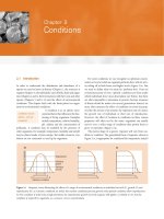
Figure 9.1 (a) Phlorotannin content of Ascophyllum nodosum
plants after exposure to simulated herbivory (removing tissue with
a hole punch) or grazing by real herbivores of two species. Means
and standard errors are shown. Only the snail Littorina obtusata
had the effect of inducing increased concentrations of the
defensive chemical in the seaweed. Different letters indicate that
means are significantly different (P < 0.05). (b) In a subsequent

experiment, the snails were presented with algal shoots from
the control and snail-grazed treatments in (a); the snails ate
significantly less of plants with a high phlorotannin content.
(After Pavia & Toth 2000.)
Leaf area damaged (%)
Apr 6
0
5
10
15
Apr 20
(a)
Number of aphids per plant
Apr 6
0
10
30
Apr 20
(b)
Plant fitness
(seeds × seed mass)
Treatment
0
1
2
3
(c)
20
40
Control

Damage
control
Induced
Sampling date
Figure 9.2 (a) Percentage of leaf area consumed by chewing
herbivores and (b) number of aphids per plant, measured on
two dates (April 6 and April 20) in three field treatments: overall
control, damage control (tissue removed by scissors) and induced
(caused by grazing of caterpillars of Pieris rapae). (c) The fitness
of plants in the three treatments calculated by multiplying the
number of seeds produced by the mean seed mass (in mg).
(After Agrawal, 1998.)
EIPC09 10/24/05 2:01 PM Page 269
270 CHAPTER 9
phenotype that is best for that set of conditions) (Karban et al.,
1999). Of course, it is not only the costs of inducible defenses that
can be set against fitness benefits. Constitutive defenses, such as
spines, trichomes or defensive chemicals (particularly in the fam-
ilies Solanaceae and Brassicaceae), also have costs that have been
measured (in phenotypes or genotypes lacking the defense) in terms
of reductions in growth or the production of flowers, fruits or
seeds (see review by Strauss et al., 2002).
9.2.3 Herbivory, defoliation and plant growth
Despite a plethora of defensive struc-
tures and chemicals, herbivores still
eat plants. Herbivory can stop plant
growth, it can have a negligible effect on growth rate, and it can
do just about anything in between. Plant compensation may be
a general response to herbivory or may be specific to particular
herbivores. Gavloski and Lamb (2000b) tested these alternative

hypotheses by measuring the biomass of two cruciferous plants
Brassica napus and Sinapis alba in response to 0, 25 and 75%
defoliation of seedling plants by three herbivore species with
biting and chewing mouthparts – adult flea beetles Phyllotreta
cruciferae and larvae of the moths Plutella xylostella and Mamestra
configurata. Not surprisingly, both plant species compensated
better for 25% than 75% defoliation. However, although defoli-
ated to the same extent, both plants tended to compensate best
for defoliation by the moth M. configurata and least for the beetle
P. cruciferae (Figure 9.3). Herbivore-specific compensation may
reflect plant responses to slightly different patterns of defoliation
or different chemicals in saliva that suppress growth in contrasting
ways (Gavloski & Lamb, 2000b).
••••
Compensation index
–2.0
–1.5
–1.0
–0.5
0.0
0.5
B. napus: 25%
Compensation index
–2.0
–1.5
–1.0
–0.5
0.0
0.5
B. napus: 75%

*
Compensation index
–2.0
–1.5
–1.0
–0.5
0.0
0.5
S. alba: 25%
7 14 21 28
Days after defoliation
Compensation index
–2.0
–1.5
–1.0
–0.5
0.0
0.5
S. alba: 75%
7 142128
Days after defoliation
Phyllotreta cruciferae
Plutella xylostella
Mamestra configurata
*
*
*
*
*
*

Figure 9.3 Compensation of leaf biomass
(mean ± SE: (log
e
biomass defoliated plant)
– (log
e
of mean for control plants)) of
Brassica napus and Sinapis alba seedlings
with 25 or 75% defoliation by three
species of insect (see key) in a controlled
environment. On the vertical axis, zero
equates to perfect compensation, negative
values to undercompensation and positive
values to overcompensation. Mean
biomasses of defoliated plants that differ
significantly from corresponding controls
are indicated by an asterisk. (After Gavloski
& Lamb, 2000b.)
timing of herbivory
is crucial
EIPC09 10/24/05 2:01 PM Page 270
THE NATURE OF PREDATION 271
In the example above, compensation, which was generally
complete by 21 days after defoliation, was associated with changes
in root biomass consistent with the maintenance of a constant
shoot : root ratio. Many plants compensate for herbivory in this
way by altering the distribution of photosynthate in different parts
of the plant. Thus, for example, Kosola et al. (2002) found that
the concentration of soluble sugars in the young (white) fine roots
of poplars (Populus canadensis) defoliated by gypsy moth caterpil-

lars (Lymantria dispar) was much lower than in undefoliated
trees. Older roots (>1 month in age), on the other hand, showed
no significant effect of defoliation.
Often, there is considerable difficulty in assessing the real
extent of defoliation, refoliation and hence net growth. Close
monitoring of waterlily leaf beetles (Pyrrhalta nymphaeae) grazing
on waterlilies (Nuphar luteum) revealed that leaves were rapidly
removed, but that new leaves were also rapidly produced. More
than 90% of marked leaves on grazed plants had disappeared within
17 days, while marked leaves on ungrazed plants were still com-
pletely intact (Figure 9.4). However, simple counts of leaves on
grazed and ungrazed plants only indicated a 13% loss of leaves
to the beetles, because of new leaf production on grazed plants.
The plants that seem most tolerant
of grazing, especially vertebrate grazing,
are the grasses. In most species, the
meristem is almost at ground level
amongst the basal leaf sheaths, and
this major point of growth (and regrowth) is therefore usually
protected from grazers’ bites. Following defoliation, new leaves
are produced using either stored carbohydrates or the photosyn-
thate of surviving leaves, and new tillers are also often produced.
Grasses do not benefit directly from their grazers’ attentions.
But it is likely that they are helped by grazers in their competit-
ive interactions with other plants (which are more strongly
affected by the grazers), accounting for the predominance of
grasses in so many natural habitats that suffer intense vertebrate
grazing. This is an example of the most widespread reason for
herbivory having a more drastic effect on grazing-intolerant
species than is initially apparent – the interaction between

herbivory and plant competition (the range of possible con-
sequences of which are discussed by Pacala & Crawley, 1992;
see also Hendon & Briske, 2002). Note also that herbivores can
have severe nonconsumptive effects on plants when they act
as vectors for plant pathogens (bacteria, fungi and especially
viruses) – what the herbivores take from the plant is far less import-
ant than what they give it! For instance, scolytid beetles feeding
on the growing twigs of elm trees act as vectors for the fungus
that causes Dutch elm disease. This killed vast numbers of elms
in northeastern USA in the 1960s, and virtually eradicated them
in southern England in the 1970s and early 1980s.
9.2.4 Herbivory and plant survival
Generally, it is more usual for herbivores
to increase a plant’s susceptibility to
mortality than to kill it outright. For
example, although the flea beetle
Altica sublicata reduced the growth rate of the sand-dune willow
Salix cordata in both 1990 and 1991 (Figure 9.5), significant
mortality as a result of drought stress only occurred in 1991.
Then, however, susceptibility was strongly influenced by the
herbivore: 80% of plants died in a high herbivory treatment
(eight beetles per plant), 40% died at four beetles per plant, but
none of the beetle-free control plants died (Bach, 1994).
Repeated defoliation can have an
especially drastic effect. Thus, a single
defoliation of oak trees by the gypsy
moth (Lymantria dispar) led to only a 5%
mortality rate whereas three succes-
sive heavy defoliations led to mortality rates of up to 80%
(Stephens, 1971). The mortality of established plants, however,

is not necessarily associated with massive amounts of defoliation.
One of the most extreme cases where the removal of a small
amount of plant has a disproportionately profound effect is
ring-barking of trees, for example by squirrels or porcupines. The
cambial tissues and the phloem are torn away from the woody
xylem, and the carbohydrate supply link between the leaves
and the roots is broken. Thus, these pests of forestry plantations
often kill young trees whilst removing very little tissue. Surface-
feeding slugs can also do more damage to newly established
grass populations than might be expected from the quantity of
material they consume (Harper, 1977). The slugs chew through
••••
Ungrazed Grazed
17
0
1
80
100
11
(Jul 26)
4
(Aug 11)
Days since marking
60
40
20
Leaf area remaining (%)
Figure 9.4 The survivorship of leaves on waterlily plants grazed
by the waterlily leaf beetle was much lower than that on ungrazed
plants. Effectively, all leaves had disappeared at the end of 17 days,

despite the fact that ‘snapshot’ estimates of loss rates to grazing on
grazed plants during this period suggested only around a 13% loss.
(After Wallace & O’Hop, 1985.)
grasses are
particularly tolerant
of grazing
mortality: the result
of an interaction with
another factor?
repeated defoliation
or ring-barking
can kill
EIPC09 10/24/05 2:01 PM Page 271
272 CHAPTER 9
the young shoots at ground level, leaving the felled leaves
uneaten on the soil surface but consuming the meristematic
region at the base of shoots from which regrowth would occur.
They therefore effectively destroy the plant.
Predation of seeds, not surprisingly, has a predictably
harmful effect on individual plants (i.e. the seeds themselves).
Davidson et al. (1985) demonstrated dramatic impacts of seed-
eating ants and rodents on the composition of seed banks of ‘annual’
plants in the deserts of southwestern USA and thus on the make
up of the plant community.
9.2.5 Herbivory and plant fecundity
The effects of herbivory on plant
fecundity are, to a considerable extent,
reflections of the effects on plant
growth: smaller plants bear fewer seeds.
However, even when growth appears

to be fully compensated, seed produc-
tion may nevertheless be reduced because of a shift of resources
from reproductive output to shoots and roots. This was the
case in the study shown in Figure 9.3 where compensation in
growth was complete after 21 days but seed production was still
significantly lower in the herbivore-damaged plants. Moreover,
indirectly through its effect on leaf area, or by directly feeding
on reproductive structures, herbivory can affect floral traits
(corolla diameter, floral tube length, flower number) and have
an adverse impact on pollination and seed set (Mothershead &
Marquis, 2000). Thus experimentally ‘grazed’ plants of Oenothera
macrocarpa produced 30% fewer flowers and 33% fewer seeds.
Plants may also be affected more
directly, by the removal or destruction
of flowers, flower buds or seeds. Thus,
caterpillars of the large blue butterfly
Maculinea rebeli feed only in the flowers
and on the fruits of the rare plant
Gentiana cruciata, and the number of seeds per fruit (70 compared
to 120) is reduced where this specialist herbivore occurs (Kery
et al., 2001). Many studies, involving the artificial exclusion or
removal of seed predators, have shown a strong influence of
predispersal seed predation on recruitment and the density
of attacked species. For example, seed predation was a significant
factor in the pattern of increasing abundance of the shrub
Haplopappus squarrosus along an elevational gradient from the
Californian coast, where predispersal seed predation was higher,
to the mountains (Louda, 1982); and restriction of the crucifer
Cardamine cordifolia to shaded situations in the Rocky Mountains
was largely due to much higher levels of predispersal seed pre-

dation in unshaded locations (Louda & Rodman, 1996).
It is important to realize, however,
that many cases of ‘herbivory’ of reprod-
uctive tissues are actually mutualistic,
benefitting both the herbivore and the
plant (see Chapter 13). Animals that
‘consume’ pollen and nectar usually transfer pollen inadvertently
from plant to plant in the process; and there are many fruit-
eating animals that also confer a net benefit on both the parent
••••
No herbivory
Low herbivory
High herbivory
Clone number
41
0.8
32
Relative change in height
0.6
0.4
0.2
0.0
5 6
0.6
87
0.4
0.2
0.0
9
(b) Aug 10 – Aug 21(a) Jul 19 – Aug 17

Figure 9.5 Relative growth rates (changes in height, with standard errors) of a number of different clones of the sand-dune willow,
Salix cordata, (a) in 1990 and (b) in 1991, subjected either to no herbivory, low herbivory (four flea beetles per plant) or high herbivory
(eight beetles per plant). (After Bach, 1994.)
herbivores affect
plant growth . . .
. . . indirectly by
reducing seed
production . . .
and directly
by removing
reproductive
structures
much pollen and
fruit herbivory
benefits the plant
EIPC09 10/24/05 2:01 PM Page 272
THE NATURE OF PREDATION 273
plant and the individual seed within the fruit. Most vertebrate fruit-
eaters, in particular, either eat the fruit but discard the seed, or
eat the fruit but expel the seed in the feces. This disperses the seed,
rarely harms it and frequently enhances its ability to germinate.
Insects that attack fruit or developing fruit, on the other
hand, are very unlikely to have a beneficial effect on the plant.
They do nothing to enhance dispersal, and they may even make
the fruit less palatable to vertebrates. However, some large ani-
mals that normally kill seeds can also play a part in dispersing them,
and they may therefore have at least a partially beneficial effect.
There are some ‘scatter-hoarding’ species, like certain squirrels,
that take nuts and bury them at scattered locations; and there are
other ‘seed-caching’ species, like some mice and voles, that collect

scattered seeds into a number of hidden caches. In both cases,
although many seeds are eaten, the seeds are dispersed, they are
hidden from other seed predators and a number are never
relocated by the hoarder or cacher (Crawley, 1983).
Herbivores also influence fecundity in a number of other
ways. One of the most common responses to herbivore attack is
a delay in flowering. For instance, in longer lived semelparous
species, herbivory frequently delays flowering for 1 year or
more, and this typically increases the longevity of such plants since
death almost invariably follows their single burst of reproduction
(see Chapter 4). Poa annua on a lawn can be made almost
immortal by mowing it at weekly intervals, whereas in natural
habitats, where it is allowed to flower, it is commonly an annual
– as its name implies.
Generally, the timing of defoliation
is critical in determining the effect on
plant fecundity. If leaves are removed
before inflorescences are formed, then the extent to which
fecundity is depressed clearly depends on the extent to which the
plant is able to compensate. Early defoliation of a plant with sequen-
tial leaf production may have a negligible effect on fecundity;
but where defoliation takes place later, or where leaf production
is synchronous, flowering may be reduced or even inhibited
completely. If leaves are removed after the inflorescence has
been formed, the effect is usually to increase seed abortion or to
reduce the size of individual seeds.
An example where timing is important is provided by field gen-
tians (Gentianella campestris). When herbivory on this biennial plant
is simulated by clipping to remove half its biomass (Figure 9.6a),
the outcome depends on the timing of the clipping (Figure 9.6b).

Fruit production was much increased over controls if clipping
••••
Unclipped Clipped
Before clipping
(a)
(b)
Jul 12
0
Control
30
Number of fruits
25
20
15
10
5
Jul 20
Jul 28
a
b
c
d
the timing of
herbivory is critical
Figure 9.6 (a) Clipping of field gentians
to simulate herbivory causes changes in
the architecture and numbers of flowers
produced. (b) Production of mature (open
histograms) and immature fruits (black
histograms) of unclipped control plants and

plants clipped on different occasions from
July 12 to 28, 1992. Means and standard
errors are shown and all means are
significantly different from each other
(P < 0.05). Plants clipped on July 12 and
20 developed significantly more fruits than
unclipped controls. Plants clipped on July
28 developed significantly fewer fruits than
controls. (After Lennartsson et al., 1998).
EIPC09 10/24/05 2:01 PM Page 273
274 CHAPTER 9
occurred between 1 and 20 July, but if clipping occurred later than
this, fruit production was less in the clipped plants than in the
unclipped controls. The period when the plants show compen-
sation coincides with the time when damage by herbivores nor-
mally occurs.
9.2.6 A postscript: antipredator chemical defenses
in animals
It should not be imagined that antipred-
ator chemical defenses are restricted to
plants. A variety of constitutive animal
chemical defenses were described in Chapter 3 (see Section 3.7.4),
including plant defensive chemicals sequestered by herbivores from
their food plants (see Section 3.7.4). Chemical defenses may
be particularly important in modular animals, such as sponges,
which lack the ability to escape from their predators. Despite their
high nutritional value and lack of physical defenses, most marine
sponges appear to be little affected by predators (Kubanek et al.,
2002). In recent years, several triterpene glycosides have been
extracted from sponges, including from Ectyoplasia ferox in the

Caribbean. In a field study, crude extracts of refined triterpene
glycosides from this sponge were presented in artificial food
substrates to natural assemblages of reef fishes in the Bahamas.
Strong antipredatory affects were detected when compared to
control substrates (Figure 9.7). It is of interest that the triterpene
glycosides also adversely affected competitors of the sponge, includ-
ing ‘fouling’ organisms that overgrow them (bacteria, invertebrates
and algae) and other sponges (an example of allelopathy – see
Section 8.3.2). All these enemies were apparently deterred by
surface contact with the chemicals rather than by water-borne
effects (Kubanek et al., 2002).
9.3 The effect of predation on prey populations
Returning now to predators in general, it may seem that
since the effects of predators are harmful to individual prey, the
immediate effect of predation on a population of prey must also
be predictably harmful. However, these effects are not always so
predictable, for one or both of two important reasons. In the first
place, the individuals that are killed (or harmed) are not always
a random sample of the population as a whole, and may be those
with the lowest potential to contribute to the population’s future.
Second, there may be compensatory changes in the growth, sur-
vival or reproduction of the surviving prey: they may experience
reduced competition for a limiting resource, or produce more off-
spring, or other predators may take fewer of the prey. In other
words, whilst predation is bad for the prey that get eaten, it may
be good for those that do not. Moreover, predation is least likely
to affect prey dynamics if it occurs at a stage of the prey’s life
cycle that does not have a significant effect, ultimately, on prey
abundance.
To deal with the second point first,

if, for example, plant recruitment is
not limited by the number of seeds
produced, then insects that reduce
seed production are unlikely to have an important effect on
plant abundance (Crawley, 1989). For instance, the weevil
Rhinocyllus conicus does not reduce recruitment of the nodding
thistle, Carduus nutans, in southern France despite inflicting
seed losses of over 90%. Indeed, sowing 1000 thistle seeds per
square meter also led to no observable increase in the number
of thistle rosettes. Hence, recruitment appears not to be limited
by the number of seeds produced; although whether it is
limited by subsequent predation of seeds or early seedlings, or
the availability of germination sites, is not clear (Crawley, 1989).
(However, we have seen in other situations (see Section 9.2.5)
that predispersal seed predation can profoundly affect seed-
ling recruitment, local population dynamics and variation in
relative abundance along environmental gradients and across
microhabitats.)
The impact of predation is often
limited by compensatory reactions
amongst the survivors as a result of
reduced intraspecific competition. Thus,
in a classic experiment in which large numbers of woodpigeons
(Columba palumbus) were shot, the overall level of winter mor-
tality was not increased, and stopping the shooting led to no
increase in pigeon abundance (Murton et al., 1974). This was
because the number of surviving pigeons was determined ultimately
not by shooting but by food availability, and so when shooting
reduced density, there were compensatory reductions in intra-
specific competition and in natural mortality, as well as density-

dependent immigration of birds moving in to take advantage of
unexploited food.
••••
% eaten
0
100
Control
(a)
Treated
80
60
40
20
0
100
Control
(b)
Treated
80
60
40
20
Figure 9.7 Results of field assays assessing antipredatory effects
of compounds from the sponge Ectyoplasia ferox against natural
assemblages of reef fish in the Bahamas. Means (+ SE) are shown
for percentages of artificial food substrates eaten in controls
(containing no sponge extracts) in comparison with: (a) substrates
containing a crude sponge extract (t-test, P = 0.036) and
(b) substrates containing triterpene glycosides from the sponge
(P = 0.011). (After Kubanek et al., 2002.)

animals also defend
themselves
predation may occur
at a demographically
unimportant stage
compensatory
reactions amongst
survivors
EIPC09 10/24/05 2:01 PM Page 274
THE NATURE OF PREDATION 275
Indeed, whenever density is high
enough for intraspecific competition
to occur, the effects of predation on a
population should be ameliorated by the
consequent reductions in intraspecific competition. Outcomes of
predation may, therefore, vary with relative food availability. Where
food quantity or quality is higher, a given level of predation may
not lead to a compensatory response because prey are not food-
limited. This hypothesis was tested by Oedekoven and Joern
(2000) who monitored grasshopper (Ageneotettix deorum) sur-
vivorship in caged prairie plots subject to fertilization (or not)
to increase food quality in the presence or absence of lycosid
spiders (Schizocoza spp.). With ambient food quality (no fertilizer,
black symbols), spider predation and food limitation were com-
pensatory: the same numbers of grasshoppers were recovered
at the end of the 31-day experiment (Figure 9.8). However, with
higher food quality (nitrogen fertilizer added, colored symbols),
spider predation reduced the numbers surviving compared to the
no-spider control: a noncompensatory response. Under ambient
conditions after spider predation, the surviving grasshoppers

encountered more food per capita and lived longer as a result of
reduced competition. However, grasshoppers were less food-
limited when food quality was higher so that after predation the
release of additional per capita food did not promote survivor-
ship (Oedekoven & Joern, 2000).
Turning to the nonrandom distribu-
tion of predators’ attention within
a population of prey, it is likely, for
example, that predation by many large
carnivores is focused on the old (and
infirm), the young (and naive) or the sick. For instance, a study
in the Serengeti found that cheetahs and wild dogs killed a dispro-
portionate number from the younger age classes of Thomson’s
gazelles (Figure 9.9a), because: (i) these young animals were
easier to catch (Figure 9.9b); (ii) they had lower stamina and
running speeds; (iii) they were less good at outmaneuvering
the predators (Figure 9.9c); and (iv) they may even have failed
to recognize the predators (FitzGibbon & Fanshawe, 1989;
FitzGibbon, 1990). Yet these young gazelles will also have been
making no reproductive contribution to the population, and the
effects of this level of predation on the prey population will
therefore have been less than would otherwise have been the case.
Similar patterns may also be found in plant populations. The
mortality of mature Eucalyptus trees in Australia, resulting from
defoliation by the sawfly Paropsis atomaria, was restricted almost
entirely to weakened trees on poor sites, or to trees that had
suffered from root damage or from altered drainage following
cultivation (Carne, 1969).
Taken overall, then, it is clear that
the step from noting that individual

prey are harmed by individual predators
to demonstrating that prey adundance
is adversely affected is not an easy one to take. Of 28 studies in
which herbivorous insects were experimentally excluded from plant
communities using insecticides, 50% provided evidence of an effect
on plants at the population level (Crawley, 1989). As Crawley noted,
however, such proportions need to be treated cautiously. There is
an almost inevitable tendency for ‘negative’ results (no popula-
tion effect) to go unreported, on the grounds of there being
‘nothing’ to report. Moreover, the exclusion studies often took
7 years or more to show any impact on the plants: it may be
that many of the ‘negative’ studies were simply given up too early.
••••
No spiders, no fertilizer
No spiders, fertilizer
Spiders, no fertilizer
Spiders, fertilizer
Log
e
(number of grasshoppers)
20155
0
0
1
2
3
10
Time (days)
25 30 35
Figure 9.8 Trajectories of numbers

of grasshoppers surviving (mean ± SE)
for fertilizer and predation treatment
combinations in a field experiment
involving caged plots in the Arapaho
Prairie, Nebraska, USA. (After
Oedekoven & Joern, 2000.)
effects ameliorated
by reduced
competition
predatory attacks are
often directed at the
weakest prey
difficulties of
demonstrating effects
on prey populations
EIPC09 10/24/05 2:01 PM Page 275
••
276 CHAPTER 9
Many more recent investigations have shown clear effects of seed
predation on plant abundance (e.g. Kelly & Dyer, 2002; Maron
et al., 2002).
9.4 Effects of consumption on consumers
The beneficial effects that food has on
individual predators are not difficult
to imagine. Generally speaking, an
increase in the amount of food con-
sumed leads to increased rates of
growth, development and birth, and decreased rates of mortal-
ity. This, after all, is implicit in any discussion of intraspecific
competition amongst consumers (see Chapter 5): high densities,

implying small amounts of food per individual, lead to low
growth rates, high death rates, and so on. Similarly, many of the
effects of migration previously considered (see Chapter 6) reflect
the responses of individual consumers to the distribution of food
availability. However, there are a number of ways in which the
relationships between consumption rate and consumer benefit
can be more complicated than they initially appear. In the first
place, all animals require a certain amount of food simply for
maintenance and unless this threshold is exceeded the animal
will be unable to grow or reproduce, and will therefore be
unable to contribute to future generations. In other words, low
consumption rates, rather than leading to a small benefit to the
consumer, simply alter the rate at which the consumer starves
to death.
At the other extreme, the birth,
growth and survival rates of individual
consumers cannot be expected to rise
indefinitely as food availability is increased. Rather, the con-
sumers become satiated. Consumption rate eventually reaches a
plateau, where it becomes independent of the amount of food avail-
able, and benefit to consumers therefore also reaches a plateau.
Thus, there is a limit to the amount that a particular consumer
population can eat, a limit to the amount of harm that it can
do to its prey population at that time, and a limit to the extent
by which the consumer population can increase in size. This is
discussed more fully in Section 10.4.
The most striking example of whole
populations of consumers being sati-
ated simultaneously is provided by
the many plant species that have mast

years. These are occasional years in which there is synchronous
production of a large volume of seed, often across a large geo-
graphic area, with a dearth of seeds produced in the years in
between (Herrera et al., 1998; Koenig & Knops, 1998; Kelly et al.,
2000). This is seen particularly often in tree species that suffer gen-
erally high intensities of seed predation (Silvertown, 1980) and it
is therefore especially significant that the chances of escaping seed
predation are likely to be much higher in mast years than in other
years. Masting seems to be especially common in the New
Zealand flora (Kelly, 1994) where it has also been reported for
tussock grass species (Figure 9.10). The individual predators of seeds
are satiated in mast years, and the populations of predators can-
not increase in abundance rapidly enough to exploit the glut. This
••
Percentage
0
Fawns
40
60
80
(a)
20
Half-growns
Adolescents
Sub-adults
Adults
Killed by cheetahs
Killed by wild dogs
Percentage in population
Percentage of chased

gazelles escaping
0
Fawns
40
60
80
(b)
20
Half-growns
Adolescents
Distance lost (m)
–1.5
Fawns
0.0
1.0
2.0
(c)
–1.0
Half-growns and
adolescents
Adults
–0.5
0.5
1.5
Figure 9.9 (a) The proportions of different age classes (determined by tooth wear) of Thomson’s gazelles in cheetah and wild dog kills is
quite different from their proportions in the population as a whole. (b) Age influences the probability for Thomson’s gazelles of escaping
when chased by cheetahs. (c) When prey (Thomson’s gazelles) ‘zigzag’ to escape chasing cheetahs, prey age influences the mean distance
lost by the cheetahs. (After FitzGibbon & Fanshawe, 1989; FitzGibbon, 1990.)
consumers often
need to exceed

a threshold of
consumption
consumers may
become satiated
mast years and the
satiation of seed
predators
EIPC09 10/24/05 2:01 PM Page 276
••
THE NATURE OF PREDATION 277
is illustrated in Figure 9.11 where the percentage of florets of the
grass Chionochloa pallens attacked by insects remains below 20%
in mast years but ranges up to 80% or more in nonmast years.
The fact that C. pallens and four other species of Chionochloa show
strong synchrony in masting is likely to result in an increased benefit
to each species in terms of escaping seed predation in mast years.
On the other hand, the production of a mast crop makes great
demands on the internal resources of a plant. A spruce tree in a
mast year averages 38% less annual growth than in other years,
and the annual ring increment in forest trees may be reduced by
as much during a mast year as by a heavy attack of defoliating
caterpillars. The years of seed famine are therefore essentially years
of plant recovery.
As well as illustrating the potential
importance of predator satiation, the
example of masting highlights a further
point relating to timescales. The seed
predators are unable to extract the
maximum benefit from (or do the maximum harm to) the mast
crop because their generation times are too long. A hypothetical

seed predator population that could pass through several gener-
ations during a season would be able to increase exponentially
and explosively on the mast crop and destroy it. Generally speak-
ing, consumers with relatively short generation times tend to closely
track fluctuations in the quantity or abundance of their food or
••
Flowering intensity
(inflorescences tussock
–1
)
19951985
0
1975
10
20
30
1980
5
15
25
1990
C. rubra
C. seretofolia
C. rigida
Flowering intensity
(inflorescences tussock
–1
)
19951985
0

1975
4
6
8
1980
Year
1990
2
C. crassiuscula
C. palliens
Mast years
0
20
Nonmast years
40
60
80
Insect predation
(% florets attacked)
Figure 9.10 The flowering rate for five
species of tussock grass (Chionochloa)
between 1973 and 1996 in Fiordland
National Park, New Zealand. Mast years
are highly synchronized in the five species,
seemingly in response to high temperatures
in the previous season, when flowering is
induced. (After McKone et al., 1998.)
Figure 9.11 Insect predation on florets of Chionochloa pallens
in mast (n = 3) and nonmast years (n = 7) from 1988 to 1997 at
Mount Hutt, New Zealand. A mast year is defined here as one

with greater than 10 times as many florets produced per tussock
than in the previous year. The significant difference in insect
damage supports the hypothesis that the function of masting is
to satiate seed predators. (After McKone et al., 1998.)
a consumer’s
numerical response
is limited by its
generation time . . .
EIPC09 10/24/05 2:01 PM Page 277
278 CHAPTER 9
prey, whereas consumers with relatively long generation times
take longer to respond to increases in prey abundance, and
longer to recover when reduced to low densities.
The same phenomenon occurs in
desert communities, where year-to-
year variations in precipitation can be
both considerable and unpredictable,
leading to similar year-to-year variation in the productivity of many
desert plants. In the rare years of high productivity, herbivores
are typically at low abundance following one or more years of
low plant productivity. Thus, the herbivores are likely to be sati-
ated in such years, allowing plant populations to add consider-
ably to their reserves, perhaps by augmenting their buried seed
banks or their underground storage organs (Ayal, 1994). The ex-
ample of fruit production by Asphodelus ramosus in the Negev desert
in Israel in shown in Figure 9.12. The mirid bug, Capsodes infus-
catus, feeds on Asphodelus, exhibiting a particular preference for
the developing flowers and young fruits. Potentially, therefore,
it can have a profoundly harmful effect on the plant’s fruit
production. But it only passes through one generation per year.

Hence, its abundance tends never to match that of its host plant
(Figure 9.12). In 1988 and 1991, fruit production was high but
mirid abundance was relatively low: the reproductive output
of the mirids was therefore high (3.7 and 3.5 nymphs per adult,
respectively), but the proportion of fruits damaged was relatively
low (0.78 and 0.66). In 1989 and 1992, on the other hand, when
fruit production had dropped to much lower levels, the propor-
tion of fruits damaged was much higher (0.98 and 0.87) and the
reproductive output was lower (0.30 nymphs per adult in 1989;
unknown in 1992). This suggests that herbivorous insects, at least,
may have a limited ability to affect plant population dynamics
in desert communities, but that the potential is much greater for
the dynamics of herbivorous insects to be affected by their food
plants (Ayal, 1994).
Chapter 3 stressed that the quantity
of food consumed may be less import-
ant than its quality. In fact, food qual-
ity, which has both positive aspects
(like the concentrations of nutrients)
and negative aspects (like the concentrations of toxins), can only
sensibly be defined in terms of the effects of the food on the
animal that eats it; and this is particularly pertinent in the case
of herbivores. For instance, we saw in Figure 9.8 how even in
the presence of predatory spiders, enhanced food quality led to
increased survivorship of grasshoppers. Along similar lines,
Sinclair (1975) examined the effects of grass quality (protein con-
tent) on the survival of wildebeest in the Serengeti of Tanzania.
Despite selecting protein-rich plant material (Figure 9.13a), the
wildebeest consumed food in the dry season that contained well
below the level of protein necessary even for maintenance (5–6%

of crude protein); and to judge by the depleted fat reserves of dead
males (Figure 9.13b), this was an important cause of mortality.
Moreover, it is highly relevant that the protein requirements of
females during late pregnancy and lactation (December–May in
the wildebeest) are three to four times higher than the normal.
It is therefore clear that the shortage of high-quality food (and
not just food shortage per se) can have a drastic effect on the growth,
survival and fecundity of a consumer. In the case of herbivores
especially, it is possible for an animal to be apparently surrounded
by its food whilst still experiencing a food shortage. We can see
the problem if we imagine that we ourselves are provided with
a perfectly balanced diet – diluted in an enormous swimming pool.
The pool contains everything we need, and we can see it there
before us, but we may very well starve to death before we can
drink enough water to extract enough nutrients to sustain our-
selves. In a similar fashion, herbivores may frequently be confronted
with a pool of available nitrogen that is so dilute that they have
difficulty processing enough material to extract what they need.
Outbreaks of herbivorous insects may then be associated with rare
elevations in the concentration of available nitrogen in their food
plants (see Section 3.7.1), perhaps associated with unusually dry
or, conversely, unusually waterlogged conditions (White, 1993).
Consumers obviously need to acquire resources – but, to benefit
from them fully they need to acquire them in appropriate quant-
ities and in an appropriate form. The behavioral strategies that
have evolved in the face of the pressures to do this are the main
topic of the next two sections.
9.5 Widths and compositions of diets
Consumers can be classified as either
monophagous (feeding on a single

prey type), oligophagous (few prey
types) or polyphagous (many prey
types). An equally useful distinction is
••••
Number of individuals (1000s)
939290
0
87
2.1
2.8
3.5
91
Year
1.4
0.7
88 89
Number of fruits (1000s)
0
30
20
10
Figure 9.12 Fluctuations in the fruit production of Asphodelus (᭿)
and the number of Capsodes nymphs (
᭹) and adults (᭡) at a study
site in the Negev desert, Israel. (After Ayal, 1994.)
. . . as illustrated by
desert interactions
food quality rather
than quantity can
be of paramount

importance
range and
classification of
diet widths
EIPC09 10/24/05 2:01 PM Page 278
THE NATURE OF PREDATION 279
between specialists (broadly, monophages and oligophages) and
generalists (polyphages). Herbivores, parasitoids and true preda-
tors can all provide examples of monophagous, oligophagous and
polyphagous species. But the distribution of diet widths differs
amongst the various types of consumer. True predators with spe-
cialized diets do exist (for instance the snail kite Rostrahamus socia-
bilis feeds almost entirely on snails of the genus Pomacea), but most
true predators have relatively broad diets. Parasitoids, on the other
hand, are typically specialized and may even be monophagous.
Herbivores are well represented in all categories, but whilst
grazing and ‘predatory’ herbivores typically have broad diets, ‘par-
asitic’ herbivores are very often highly specialized. For instance,
Janzen (1980) examined 110 species of beetle that feed as larvae
inside the seeds of dicotyledonous plants in Costa Rica (‘parasitizing’
them) and found that 83 attacked only one plant species, 14
attacked only two, nine attacked three, two attacked four, one
attacked six and one attacked eight of the 975 plants in the area.
9.5.1 Food preferences
It must not be imagined that poly-
phagous and oligophagous species are
indiscriminate in what they choose
from their acceptable range. On the
contrary, some degree of preference is almost always apparent.
An animal is said to exhibit a preference for a particular type of

food when the proportion of that type in the animal’s diet is higher
than its proportion in the animal’s environment. To measure
food preference in nature, therefore, it is necessary not only to
examine the animal’s diet (usually by the analysis of gut contents)
but also to assess the ‘availability’ of different food types. Ideally,
this should be done not through the eyes of the observer (i.e. not
by simply sampling the environment), but through the eyes of
the animal itself.
A food preference can be expressed in two rather different con-
texts. There can be a preference for items that are the most valu-
able amongst those available or for items that provide an integral
part of a mixed and balanced diet. These will be referred to as
ranked and balanced preferences, respectively. In the terms of
Chapter 3 (Section 3.8), where resources were classified, indi-
viduals exhibit ranked preferences in discriminating between re-
source types that are ‘perfectly substitutable’ and exhibit balanced
preferences between resource types that are ‘complementary’.
Ranked preferences are usually
seen most clearly amongst carnivores.
For instance, Figure 9.14 shows two
examples in which carnivores actively
selected prey items that were the most
profitable in terms of energy intake
per unit time spent dealing with (or
‘handling’) prey. Results such as these reflect the fact that a car-
nivore’s food often varies little in composition (see Section 3.7.1),
but may vary in size or accessibility. This allows a single meas-
ure (like ‘energy gained per unit handling time’) to be used to
characterize food items, and it therefore allows food items to be
ranked. In other words, Figure 9.14 shows consumers exhibiting

an active preference for food of a high rank.
••••
Crude protein (%)
0
N
5
10
20
(a)
15
DJ
FM
AMJ J ASO
Bone marrow fat (%)
0
N
50
100
(b)
DJ AMJJASO
FM
Figure 9.13 (a) The quality of food measured as percentage crude protein available to (7) and eaten by (᭹) wildebeest in the Serengeti
during 1971. Despite selection (‘eaten’ > ‘available’), the quality of food eaten fell during the dry season below the level necessary for the
maintenance of nitrogen balance (5–6% of crude protein). (b) The fat content of the bone marrow of the live male population (
7) and
those found dead from natural causes (
᭹). Vertical lines, where present, show 95% confidence limits. (After Sinclair, 1975.)
preference is defined
by comparing diet
with ‘availability’

ranked preferences
predominate when
food items can be
classified on a single
scale . . .
EIPC09 10/24/05 2:01 PM Page 279
280 CHAPTER 9
For many consumers, however,
especially herbivores and omnivores,
no simple ranking is appropriate, since
none of the available food items
matches the nutritional requirements
of the consumer. These requirements
can therefore only be satisfied either by eating large quantities
of food, and eliminating much of it in order to get a sufficient
quantity of the nutrient in most limited supply (for example
aphids and scale insects excrete vast amounts of carbon in
honeydew to get sufficient nitrogen from plant sap), or by eating
a combination of food items that between them match the con-
sumer’s requirements. In fact, many animals exhibit both sorts
of response. They select food that is of generally high quality
(so the proportion eliminated is minimized), but they also select
items to meet specific requirements. For instance, sheep and
cattle show a preference for high-quality food, selecting leaves
in preference to stems, green matter in preference to dry or
old material, and generally selecting material that is higher in
nitrogen, phosphorus, sugars and gross energy, and lower in
fiber, than what is generally available. In fact, all generalist
herbivores appear to show rankings in the rate at which they eat
different food plants when given a free choice in experimental tests

(Crawley, 1983).
On the other hand, a balanced
preference is also quite common. For
instance, the plate limpet, Acmaea
scutum, selects a diet of two species
of encrusting microalgae that contains
60% of one species and 40% of the other, almost irrespective of
the proportions in which they are available (Kitting, 1980). Whilst
caribou, which survive on lichen through the winter, develop a
sodium deficiency by the spring that they overcome by drinking
seawater, eating urine-contaminated snow and gnawing shed
antlers (Staaland et al., 1980). We have only to look at ourselves
to see an example in which ‘performance’ is far better on a
mixed diet than on a pure diet of even the ‘best’ food.
There are two other important reasons why a mixed diet may
be favored. First, consumers may accept low-quality items sim-
ply because, having encountered them, they have more to gain
by eating them (poor as they are) than by ignoring them and con-
tinuing to search. This is discussed in detail in Section 9.5.3. Second,
consumers may benefit from a mixed diet because each food type
may contain a different undesirable toxic chemical. A mixed diet
would then keep the concentrations of all of these chemicals within
acceptable limits. It is certainly the case that toxins can play an
important role in food preference. For instance, dry matter
intake by Australian ringtail possums (Pseudocheirus peregrinus) feed-
ing on Eucalyptus tree leaves was strongly negatively correlated
with the concentration of sideroxylonal, a toxin found in
Eucalyptus leaves, but was not related to nutritional character-
istics such as nitrogen or cellulose (Lawler et al., 2000).
Overall, however, it would be quite wrong to give the

impression that all preferences have been clearly linked with one
explanation or another. For example, Thompson (1988) reviewed
the relationship between the oviposition preferences of phy-
tophagous insects and the performance of their offspring on the
selected food plants in terms of growth, survival and reproduc-
tion. A number of studies have shown a good association (i.e.
females preferentially oviposit on plants where their offspring
perform best), but in many others the association is poor. In
such cases there is generally no shortage of explanations for the
apparently unsuitable behavior, but these explanations are, as yet,
often just untested hypotheses.
••••
Flies selected
Flies available
Energy gain (J s
–1
)
403010
0
0
2.0
4.0
6.0
20
Length of mussel (mm)
(a)
Number of mussels
eaten per day
5
0

4
3
2
1
7
Prey length (mm)
(b)
Energy value
8
Calories s
–1
handling time
1096
10
5
12
14
16
Frequency (%)
1096
0
5
10
30
50
7
Prey length (mm)
40
20
8

Energy
Figure 9.14 Predators eating ‘profitable’ prey, i.e. predators showing a preponderance in their diet for those prey items that provide them
with the most energy. (a) When crabs (Carcinus maenas) were presented with equal quantities of six size classes of mussels (Mytilus edulis),
they tended to show a preference for those providing the greatest energy gain (energy per unit handling time). (After Elner & Hughes,
1978.) (b) Pied wagtails (Motacilla alba yarrellii) tended to select, from scatophagid flies available, those providing the greatest energy gain
per unit handling time. (After Davies, 1977; Krebs, 1978.)
. . . but many
consumers show
a combination of
ranked and balanced
preferences
mixed diets can be
favored for a variety
of reasons
EIPC09 10/24/05 2:01 PM Page 280
THE NATURE OF PREDATION 281
9.5.2 Switching
The preferences of many consumers
are fixed; in other words, they are
maintained irrespective of the relative
availabilities of alternative food types.
But many others switch their preference,
such that food items are eaten disproportionately often when they
are common and are disproportionately ignored when they are
rare. The two types of preference are contrasted in Figure 9.15.
Figure 9.15a shows the fixed preference exhibited by predatory
shore snails when they were presented with two species of
mussel prey at a range of proportions. The line in Figure 9.15a
has been drawn on the assumption that they exhibited the same
preference at all proportions. This assumption is clearly justified:

irrespective of availability, the predatory snails showed the same
marked preference for the thin-shelled, less protected Mytilus
edulis, which they could exploit more effectively. By contrast,
Figure 9.15b shows what happened when guppies (fish) were
offered a choice between fruit-flies and tubificid worms as prey.
The guppies clearly switched their preference, and consumed a
disproportionate number of the more abundant prey type.
There are a number of situations in
which switching can arise. Probably
the most common is where different
types of prey are found in different
microhabitats, and the consumers concentrate on the most
profitable microhabitat. This was the case for the guppies in
Figure 9.15b: the fruit-flies floated at the water surface whilst the
tubificids were found at the bottom. Switching can also occur
(Bergelson, 1985) in the following situations:
1 When there is an increased probability of orientating toward
a common prey type, i.e. consumers develop a ‘search image’
for abundant food (Tinbergen, 1960) and concentrate on their
‘image’ prey to the relative exclusion of nonimage prey.
••••
M. edulis eaten (%)
1008040
0
0
40
80
100
60
M. edulis offered (%)

(a)
20
60
20
Expected if no
preference
Proportion of tubificids in diet
0.80.4
0
0
0.4
0.8
1.0
0.6
Proportion of tubificids available
(b)
0.2
0.6
0.2
Expected if no
preference
Proportion of
Gammarus eaten
1.0
0
0
1.0
Proportion of Gammarus available
(d)
0.5

0.5
Number of guppies
1.00.80.4
0
0
4
8
0.6
Proportion of tubificids in diet
(c)
2
6
0.2
Figure 9.15 Switching. (a) A lack of switching: snails exhibit a consistent preference amongst the mussels Mytilus edulis and M. californianus,
irrespective of their relative abundance (means plus standard errors). (After Murdoch & Stewart-Oaten, 1975.) (b) Switching by guppies fed
on tubificids and fruit-flies: they take a disproportionate amount of whichever prey type is the more available (means and total ranges).
(After Murdoch et al., 1975.) (c) Preferences shown by the individual guppies in (b) when offered equal amounts of the two prey types:
individuals were mostly specialists on one or other type. (d) Switching by sticklebacks fed mixtures of Gammarus and Artemia: overall they
take a disproportionate amount of whichever is more available. However, in the first series of trials, with Gammarus availability decreasing
(closed symbols), first-day trialists (
᭿) tended to take more Gammarus than third-day trialists (᭹), whereas with Gammarus availability
increasing, firsts (
4) tended to take less Gammarus than thirds (7). The effects of learning are apparent. (After Hughes & Croy, 1993.)
switching involves a
preference for food
types that are
common
when might
switching arise?
EIPC09 10/24/05 2:01 PM Page 281

282 CHAPTER 9
2 When there is an increased probability of pursuing a common
prey type.
3 When there is an increased probability of capturing a common
prey type.
4 When there is an increased efficiency in handling a common
prey type.
In each case, increasingly common prey generate increased
interest and/or success on the part of the predator, and hence an
increased rate of consumption. For instance, switching occurred
in the 15-spined stickleback, Spinachia spinachia, feeding on the
crustaceans Gammarus and Artemia as alternative prey (Figure 9.15d)
as a result of learned improvements in capturing and handling
efficiencies, especially of Gammarus. Fish were fed Gammarus for
7 days, which was then replaced in the diet, in 10% steps, with Artemia
until the diet was 100% Artemia. This diet was then maintained
for a further 7 days, when the process was reversed back down
to 100% Gammarus. Each ‘step’ itself lasted 3 days, on each of
which the fish were tested. The learning process is apparent in
Figure 9.15d in the tendency for first-day trialists to be more
influenced than third-day trialists by the previous dietary mix.
Interestingly, switching in a population often seems to be a
consequence not of individual consumers gradually changing
their preference, but of the proportion of specialists changing. Figure
9.15c shows this for the guppies. When the prey types were equally
abundant, individual guppies were not generalists – rather, there
were approximately equal numbers of fruit-fly and tubificid
specialists.
It may come as a surprise that a
plant may show behavior akin to

switching. The northern pitcher plant
Sarracenia purpurea lives in nutrient-poor bogs and fens, circum-
stances that are thought to favor carnivory in plants. Carnivorous
plants such as pitcher plants invest an excess of carbon (captured
in photosynthesis) in specialist organs for capturing invertebrate
prey (effectively nitrogen-capturing structures). Figure 9.16 shows
how relative size of the pitcher keel responded to nitrogen addi-
tion to plots in Molly Bog in Vermont, USA. The more nitrogen
that was applied, the larger the relative keel size – this corresponds
to an increase in size of the noncarnivorous keel of the pitcher
and a decrease in size of the prey-catching tube. Thus, with
increasing nitrogen levels, the capacity for carnivory decreased
while maximum photosynthesis rates increased. In effect, the plants
switched effort from nitrogen to carbon capture when more
nitrogen was available in their environment.
9.5.3 The optimal foraging approach to diet width
Predators and prey have undoubtedly
influenced one another’s evolution.
This can be seen in the distasteful or
poisonous leaves of many plants, in the spines of hedgehogs and
in the camouflage coloration of many insect prey; and it can be
seen in the stout ovipositors of wood wasps, the multichambered
stomachs of cattle and the silent approach and sensory excellence
of owls. Such specialization makes it clear, though, that no predator
can possibly be capable of consuming all types of prey. Simple
design constraints prevent shrews from eating owls (even though
shrews are carnivores) and prevent humming-birds from eating
seeds.
Even within their constraints, however, most animals con-
sume a narrower range of food types than they are morphologically

capable of consuming. In trying to understand what determines
a consumer’s actual diet within its wide potential range, ecologists
have increasingly turned to optimal foraging theory. The aim of
optimal foraging theory is to predict the foraging strategy to be
expected under specified conditions. It generally makes such pre-
dictions on the basis of a number of assumptions:
1 The foraging behavior that is
exhibited by present-day animals is
the one that has been favored by
natural selection in the past but
also most enhances an animal’s fitness at present.
2 High fitness is achieved by a high net rate of energy intake
(i.e. gross energy intake minus the energetic costs of obtain-
ing that energy).
3 Experimental animals are observed in an environment to which
their foraging behavior is suited, i.e. it is a natural environment
very similar to that in which they evolved, or an experimental
arena similar in essential respects to the natural environment.
••••
Applied N (mg l
–1
)
0.01
0.2
1
Relative keel size
0.3 0.4 0.5 0.6 0.7 0.8 0.9
0.1
a plant that ‘switches’
diet width and

evolution
Figure 9.16 The relationship between relative keel size of pitchers
of Sarracenia purpurea and nitrogen added as aerial spray in plots
at Molly Bog, Vermont. Dotted lines indicate 95% confidence
intervals. A larger relative keel size corresponds to a reduced
investment in organs of prey capture. (After Ellison & Gotelli, 2002.)
assumptions inherent
in optimal foraging
theory
EIPC09 10/24/05 2:01 PM Page 282
THE NATURE OF PREDATION 283
These assumptions will not always be justified. First, other
aspects of an organism’s behavior may influence fitness more than
optimal foraging does. For example, there may be such a premium
on the avoidance of predators that animals forage at a place and
time where the risk from predators is lower, and in consequence
gather their food less efficiently than is theoretically possible
(see Section 9.5.4). Second, and just as important, for many
consumers (particularly herbivores and omnivores) the efficient
gathering of energy may be less critical than of some other
dietary constituent (e.g. nitrogen), or it may be of prime import-
ance for the forager to consume a mixed and balanced diet. In
such cases, the value of existing optimal foraging theory is
limited. However, in circumstances where the energy maximiza-
tion premise can be expected to apply, optimal foraging theory
offers a powerful insight into the significance of the foraging
‘decisions’ that predators make (for reviews see Stephens & Krebs,
1986; Krebs & Kacelnik, 1991; Sih & Christensen, 2001).
Typically, optimal foraging theory
makes predictions about foraging beha-

vior based on mathematical models
constructed by ecological theoreticians
who are omniscient (‘all knowing’) as
far as their model systems are con-
cerned. The question therefore arises: is it necessary for a real
forager to be equally omniscient and mathematical, if it is to
adopt the appropriate, optimal strategy? The answer is ‘no’. The
theory simply says that if there is a forager that in some way (in
any way) manages to do the right thing in the right circumstances,
then this forager will be favored by natural selection; and if its
abilities are inherited, these should spread, in evolutionary time,
throughout the population.
Optimal foraging theory does not specify precisely how the
forager should make the right decisions, and it does not require
the forager to carry out the same calculations as the modeler. Later
we consider another group of ‘mechanistic’ models (see Sec-
tion 9.6.2) that attempt to show how a forager, given that it is
not omniscient, might nevertheless manage to respond by ‘rules
of thumb’ to limited environmental information and thereby
exhibit a strategy that is favored by natural selection. But it is
optimal foraging theory that predicts the nature of the strategy
that should be so favored.
The first paper on optimal foraging theory (MacArthur &
Pianka, 1966) sought to understand the determination of diet ‘width’
(the range of food types eaten by an animal) within a habitat.
Subsequently, the model was developed into a more rigorous
algebraic form, notably by Charnov (1976a). MacArthur and
Pianka argued that to obtain food, any predator must expend time
and energy, first in searching for its prey and then in handling
it (i.e. pursuing, subduing and consuming it). Whilst searching,

a predator is likely to encounter a wide variety of food items.
MacArthur and Pianka therefore saw diet width as depending on
the responses of predators once they had encountered prey.
Generalists pursue (and may then subdue and consume) a large
proportion of the prey types they encounter; specialists continue
searching except when they encounter prey of their specifically
preferred type.
The ‘problem’ for any forager is
this: if it is a specialist, then it will only
pursue profitable prey items, but it
may expend a great deal of time and energy searching for them.
Whereas if it is a generalist, it will spend relatively little time search-
ing, but it will pursue both more and less profitable types of prey.
An optimal forager should balance the pros and cons so as to max-
imize its overall rate of energy intake. MacArthur and Pianka
expressed the problem as follows: given that a predator already
includes a certain number of profitable items in its diet, should
it expand its diet (and thereby decrease its search time) by includ-
ing the next most profitable item as well?
We can refer to this ‘next most profitable’ item as the ith item.
E
i
/h
i
is then the profitability of the item, where E
i
is its energy
content, and h
i
its handling time. In addition, K/M is the average

profitability of the ‘present’ diet (i.e. one that includes all prey
types that are more profitable than i, but does not include prey
type i itself ), and O is the average search time for the present diet.
If a predator does pursue a prey item of type i, then its expected
rate of energy intake is E
i
/h
i
. But if it ignores this prey item, whilst
pursuing all those that are more profitable, then it can expect to
search for a further O, following which its expected rate of energy
intake is K/M. The total time spent in this latter case is O + M, and
so the overall expected rate of energy intake is K/(O + M). The most
profitable, optimal strategy for a predator will be to pursue the
ith item if, and only if:
E
i
/h
i
≥ K/(O + M). (9.1)
In other words, a predator should continue to add increasingly
less profitable items to its diet as long as Equation 9.1 is satisfied
(i.e. as long as this increases its overall rate of energy intake).
This will serve to maximize its overall rate of energy intake,
K/(O + M).
This optimal diet model leads to a number of predictions.
1 Predators with handling times that
are typically short compared to
their search times should be gener-
alists, because in the short time it takes them to handle a prey

item that has already been found, they can barely begin to search
for another prey item. (In terms of Equation 9.1: E
i
/h
i
is large
(h
i
is small) for a wide range of prey types, whereas K/(O + M)
is small (O is large) even for broad diets.) This prediction
seems to be supported by the broad diets of many insectivo-
rous birds feeding in trees and shrubs. Searching is always
moderately time consuming, but handling the minute insects
takes negligible time and is almost always successful. A bird,
••••
theoreticians are
omniscient
mathematicians – the
foragers need not be
to pursue or not
pursue?
searchers should be
generalists
EIPC09 10/24/05 2:01 PM Page 283
284 CHAPTER 9
therefore, has something to gain and virtually nothing to lose
by consuming an item once found, and overall profitability is
maximized by a broad diet.
2 By contrast, predators with hand-
ling times that are long relative

to their search times should be spe-
cialists. That is, if O is always small,
then K/(O + M) is similar to K/M. Thus, maximizing K/(O + M) is
much the same as maximizing K/h, which is achieved, clearly,
by including only the most profitable items in the diet. For
instance, lions live more or less constantly in sight of their prey
so that search time is negligible; handling time, on the other
hand, and particularly pursuit time, can be long (and very energy
consuming). Lions consequently specialize on prey that can
be pursued most profitably: the immature, the lame and
the old.
3 Other things being equal, a predator
should have a broader diet in an
unproductive environment (where
prey items are relatively rare and
O is relatively large) than in a pro-
ductive environment (where O is
smaller). This prediction is broadly supported by the two
examples shown in Figure 9.17: in experimental arenas, both
bluegill sunfish (Lepomis macrochirus) and great tits (Parus
major) had more specialized diets when prey density was
higher. A related result has been reported from predators in
their natural setting – brown and black bears (Ursos arctos and
U. americanus) feeding on salmon in Bristol Bay in Alaska. When
salmon availability was high, bears consumed less biomass per
captured fish, targeting energy-rich fish (those that had not
spawned) or energy-rich body parts (eggs in females, brain in
males). In essence their diet became more specialized when
prey were abundant (Gende et al., 2001).
4 Equation 9.1 depends on the pro-

fitability of the ith item (E
i
/h
i
),
depends on the profitabilities of the
items already in the diet (K/M) and
depends on the search times for
items already in the diet (O) and thus on their abundance. But
it does not depend on the search time for the ith item, s
i
. In
other words, predators should ignore insufficiently profitable
food types irrespective of their abundance. Re-examining the
examples in Figure 9.17, we can see that these both refer to
cases in which the optimal diet model does indeed predict that
the least profitable items should be ignored completely. The
foraging behavior was very similar to this prediction, but in
both cases the animals consistently took slightly more than
expected of the less profitable food types. In fact, this sort of
discrepancy has been uncovered repeatedly, and there are a
number of reasons why it may occur, which can be summar-
ized crudely by noting that the animals are not omniscient.
The optimal diet model, however, does not predict a perfect
correspondence between observation and expectation. It
predicts the sort of strategy that will be favored by natural
selection, and says that the animals that come closest to this
••••
handlers should be
specialists

specialization should
be greater in
productive
environments
the abundance of
unprofitable prey
types is irrelevant
Prediction of
optimal diet
theory
(a) Bluegill sunfish
Ratio
encountered
Observed
ratio in diet
0.80 0.4
Low density
0.80 0.4
Medium density
0.80 0.4
High density
S
M
L
S
M
L
Small prey
Medium prey
Large prey

Predicted
proportion
in diet
(b) Great tit
Proportion
encountered
Observed
proportion
in diet
0.80 0.4
Low density
S
L
S
L
Small prey
Large prey
0.80 0.4
High density I
0.80 0.4
High density II
0.80 0.4
High density III
Figure 9.17 Two studies of optimal
diet choice that show a clear but limited
correspondence with the predictions of
Charnov’s (1976a) optimal diet model.
Diets are more specialized at high prey
densities; but more low profitability items
are included than predicted by the theory.

(a) Bluegill sunfish preying on different size
classes of Daphnia: the histograms show
ratios of encounter rates with each size
class at three different densities, together
with the predicted and observed ratios in
the diet. (After Werner & Hall, 1974.)
(b) Great tits preying on large and small
pieces of mealworm. (After Krebs et al.,
1977.) The histograms in this case refer
to the proportions of the two types of
item taken. (After Krebs, 1978.)
EIPC09 10/24/05 2:01 PM Page 284
THE NATURE OF PREDATION 285
strategy will be most favored. From this point of view, the cor-
respondence between data and theory in Figure 9.17 seems
much more satisfactory. Sih and Christensen (2001) reviewed
134 studies of optimal diet theory, focusing on the question
of what factors might explain the ability of the theory to
correctly predict diets. Contrary to their a priori prediction,
forager groups (invertebrate versus ectothermic vertebrate
versus endothermic vertebrate) did not differ in the likelihood
of corroborating the theory. Their major conclusion was that
while optimal diet theory generally works well for foragers that
feed on immobile or relatively immobile prey (leaves, seeds,
mealworms, zooplankton relative to fish), it often fails to pre-
dict diets of foragers that attack mobile prey (small mammals,
fish, zooplankton relative to insect predators). This may
be because variations among mobile prey in vulnerability
(encounter rate and capture success) are often more import-
ant in determining predator diets than are variations in the active

choices of predators (Sih & Christensen, 2001).
5 Equation 9.1 also provides a context for understanding the
narrow specialization of predators that live in intimate asso-
ciation with their prey, especially where an individual pre-
dator is linked to an individual prey (e.g. many parasitoids and
parasitic herbivores – and many parasites (see Chapter 12)).
Since their whole lifestyle and life cycle are finely tuned to those
of their prey (or host), handling time (M) is low; but this pre-
cludes their being finely tuned to other prey species, for
which, therefore, handling time is very high. Equation 9.1 will
thus only apply within the specialist group, but not to any food
item outside it.
On the other hand, polyphagy has definite advantages. Search costs
(O) are typically low – food is easy to find – and an individual is
unlikely to starve because of fluctuations in the abundance of one
type of food. In addition, polyphagous consumers can, of course,
construct a balanced diet, and maintain this balance by varying
preferences to suit altered circumstances, and can avoid consuming
large quantities of a toxin produced by one of its food types. These
are considerations ignored by Equation 9.1.
Overall, then, evolution may
broaden or restrict diets. Where prey
exert evolutionary pressures demanding
specialized morphological or physio-
logical responses from the consumer,
restriction is often taken to extremes. But where consumers feed
on items that are individually inaccessible or unpredictable or
lacking in certain nutrients, the diet often remains broad. An appeal-
ing and much-discussed idea is that particular pairs of predator
and prey species have not only evolved but have coevolved.

In other words, there has been an evolutionary ‘arms race’,
whereby each improvement in predatory ability has been followed
by an improvement in the prey’s ability to avoid or resist the
predator, which has been followed by a further improvement in
predatory ability, and so on. This may itself be accompanied,
on a long-term, evolutionary timescale, by speciation, so that, for
example, related species of butterfly are associated with related
species of plants – all the species of the Heliconiini feed on mem-
bers of the Passifloracaea (Ehrlich & Raven, 1964; Futuyma & May,
1992). To the extent that coevolution occurs, it may certainly
be an additional force in favor of diet restriction. At present,
however, hard evidence for predator–prey or plant–herbivore
coevolution is proving difficult to come by (Futuyma & Slatkin,
1983; Futuyma & May, 1992).
There may seem, at first sight, to be a contradiction between
the predictions of the optimal diet model and switching. In the
latter, a consumer switches from one prey type to another as their
relative densities change. But the optimal diet model suggests that
the more profitable prey type should always be taken, irrespect-
ive of its density or the density of any alternative. Switching is
presumed to occur, however, in circumstances to which the
optimal diet model does not strictly apply. Specifically, switching
often occurs when the different prey types occupy different
microhabitats, whereas the optimal diet model predicts behavior
within a microhabitat. Moreover, most other cases of switching
involve a change in the profitabilities of items of prey as their dens-
ity changes, whereas in the optimal diet model these are constants.
Indeed, in cases of switching, the more abundant prey type is the
more profitable, and in such a case the optimal diet model predicts
specialization on whichever prey type is more profitable (that is,

whichever is more abundant; in other words, switching).
9.5.4 Foraging in a broader context
It is worth stressing that foraging strat-
egies will not always be strategies for
simply maximizing feeding efficiency.
On the contrary, natural selection will
favor foragers that maximize their net
benefits, and strategies will therefore
often be modified by other, conflicting demands on the indi-
viduals concerned. In particular, the need to avoid predators will
frequently affect an animal’s foraging behavior.
This has been shown in work on foraging by nymphs of
an aquatic insect predator, the backswimmer Notonecta hoffmanni
(Sih, 1982). These animals pass through five nymphal instars
(with I being the smallest and youngest, and V the oldest), and
in the laboratory the first three instars are liable to be preyed
upon by adults of the same species, such that the relative risk of
predation from adults was:
I > II > III > IV = V ≅ no risk.
These risks appear to modify the behavior of the nymphs, in that
they tend (both in the laboratory and in the field) to avoid the
••••
coevolution:
predator–prey arms
races?
backswimmers forage
suboptimally but
avoid being preyed
on
EIPC09 10/24/05 2:01 PM Page 285

286 CHAPTER 9
central areas of water bodies, where the concentration of adults
is greatest. In fact, the relative degree of avoidance was the same
as the relative risk of predation from adults:
I > II > III > IV = V ≅ no avoidance.
Yet these central areas also contain the greatest concentration
of prey items for the nymphs, and so, by avoiding predators,
nymphs of instars I and II showed a reduction in feeding rate
in the presence of adults (although those of instar III did not).
The young nymphs displayed a less than maximal feeding rate
as a result of their avoidance of predation, but an increased
survivorship.
The modifying influence of predators
on foraging behavior has also been
studied by Werner et al. (1983b) work-
ing on bluegill sunfish. They estimated the net energy returns from
foraging in three contrasting laboratory habitats – in open water,
amongst water weeds and on bare sediment – and they exam-
ined how prey densities varied in comparable natural habitats in
a lake through the seasons. They were then able to predict the
time at which the sunfish should switch between different lake
habitats so as to maximize their overall net energy returns. In the
absence of predators, three sizes of sunfish behaved as predicted
(Figure 9.18). But in a further field experiment, this time in the
presence of predatory largemouth bass, the small sunfish restricted
their foraging to the water weed habitat (Figure 9.19) (Werner
et al., 1983a). Here, they were relatively safe from predation,
although they could only achieve a markedly submaximal rate of
energy intake. By contrast, the larger sunfish are more or less safe
from predation by bass, and they continued to forage according

to the optimal foraging predictions. In a similar vein, the nymphs
of several species of algivorous mayflies largely restrict their
feeding to the hours of darkness in streams that contain brown
trout, reducing their overall feeding rates but also reducing the
risk of predation (Townsend, 2003). In the case of mammals that
feed at night, including mice, porcupines and hares, time spent
feeding may be reduced in bright moonlight when predation risk
is highest (Kie, 1999).
A foraging strategy is an integral
part of an animal’s overall pattern of
behavior. The strategy is strongly
influenced by the selective pressures favoring the maximization
of feeding efficiency, but it may also be influenced by other, pos-
sibly conflicting demands. It is also worth pointing out one other
thing. The places where animals occur, where they are maximally
••••
Predicted net
energy gain (J s
–1
)
(a)
Percentage of
total diet
15
Jul
0.2
0.8
0.6
0.4
0.2

0.8
0.6
0.4
Small Medium Large
31 15 31 15 30
Aug Sep
(b)
100
0.2
0.8
0.6
0.4
80
60
40
20
15
Jul
31 15 31 15 30
Aug Sep
100
80
60
40
20
15
Jul
31 15 31 15 30
Aug Sep
100

80
60
40
20
Open water
Sediments
Vegetation
Figure 9.18 Seasonal patterns in (a) the predicted habitat profitabilities (net rate of energy gain) and (b) the actual percentage of the
diet originating from each habitat, for three size classes of bluegill sunfish (Lepomis macrochirus). Piscivores were absent. (The ‘vegetation’
habitat is omitted from (b) for the sake of clarity – only 8–13% of the diet originated from this habitat for all size classes of fish.) There is
good correspondence between the patterns in (a) and (b). (After Werner et al., 1983b.)
. . . as do certain fish
predation and
the realized niche
EIPC09 10/24/05 2:01 PM Page 286
THE NATURE OF PREDATION 287
abundant and where they choose to feed are all key components
of their ‘realized niches’. We saw in Chapter 8 that realized
niches can be highly constrained by competitors. Here, we see
that they can also be highly constrained by predators. This is
also seen in the effects of predation by the barn owl (Tyto alba)
on the foraging behavior of three heteromyid rodents, the
Arizona pocket mouse (Perognathus amplus), Bailey’s pocket mouse
(P. baileyi) and Merriam’s kangaroo rat (Dipodomys merriami)
(Brown et al., 1988). In the presence of owls, all three species
moved to microhabitats where they were less at risk from owl
predation and where they reduced their foraging activity.
However they did so to varying extents, such that the way in
which the microhabitat was partitioned between them was quite
different in the presence and absence of owls.

9.6 Foraging in a patchy environment
For all consumers, food is distributed
patchily. The patches may be natural
and discrete physical objects: a bush
laden with berries is a patch for a fruit-eating bird; a leaf covered
with aphids is a patch for a predatory ladybird. Alternatively, a
‘patch’ may only exist as an arbitrarily defined area in an appar-
ently uniform environment; for a wading bird feeding on a sandy
beach, different 10 m
2
areas may be thought of as patches that
contain different densities of worms. In all cases though, a patch
must be defined with a particular consumer in mind. One leaf is
an appropriate patch for a ladybird, but for a larger and more active
insectivorous bird, 1 m
2
of canopy or even a whole tree may
represent a more appropriate patch.
Ecologists have been particularly interested in patch preferences
of consumers where patches vary in the density of food or prey
items they contain. There are many examples where predators
show an ‘aggregative response’, spending more time in patches
containing high densities (because these are the most profitable
patches) (Figure 9.20a–d), although such direct density dependence
is not always the case (Figure 9.20e). We deal with aggregative
responses in more detail in Chapter 10 where their importance
in population dynamics will be our focus, and particularly their
potential to lend stability to predator–prey dynamics. For now,
we concentrate on the behavior that leads to predator aggrega-
tion (Section 9.6.1), the optimal foraging approach to patch use

(Section 9.6.2) and the distribution patterns that are likely to result
when the opposing tendencies of predators to aggregate and to
interfere with each other’s foraging are both taken into account
(Section 9.6.3).
9.6.1 Behavior that leads to aggregated distributions
There are various types of behavior
underlying the aggregative responses
of consumers, but they fall into two broad categories: those
involved with the location of profitable patches, and the
responses of consumers once within a patch. The first category
includes all examples in which consumers perceive, at a distance,
the existence of heterogeneity in the distribution of their prey.
Within the second category –
responses of consumers within patches
– there are two main aspects of behav-
ior. The first is a change in the consumer’s pattern of searching
after encountering items of food. In particular, there is often a
slowing down of movement and an increased rate of turning imme-
diately following the intake of food, both of which lead to the
consumer remaining in the vicinity of its last food item (‘area-
restricted search’). Alternatively, or in addition, consumers may
simply abandon unprofitable patches more rapidly than they
abandon profitable ones. Both types of behavior were evident when
the carnivorous, net-spinning larva of the caddis-fly Plectrocnemia
conspersa feeds on chironomid (midge) larvae in a laboratory
stream. Caddis in their nets were provided with one prey item
at the beginning of the experiment and then fed daily rations of
••••
Number of fish
25

(a) Predator present
20
15
10
5
10060200 40
Percentage vegetation where sunfish
prey are taken from
80
Number of fish
0
50
(b) No predator present
45
40
35
30
25
20
15
10
5
Figure 9.19 (a) In contrast to Figure 9.18 and to (b), when
largemouth bass (which prey on small bluegill sunfish) are
present many sunfish take prey from areas where the percentage
vegetation is high and where they are relatively protected from
predation. (After Werner et al., 1983a.)
food is patchily
distributed
locating a patch

area-restricted search
EIPC09 10/24/05 2:01 PM Page 287
•• ••
288 CHAPTER 9
3010
0
0
10
30
40
20
Aphids per leaf
(a)
20
Searching time
per leaf (min)
4000
0
0
10
2000
Number of Corophium (m
–2
)
(b)
5
Number of redshank (ha
–1
)
Parasitism (%)

25155
0
0
20
40
50
10
Host density per patch
(c)
10
30
20 1000600200
0
0
20
40
60
400
Host density per patch
(d)
10
30
800
50
800600200
0
0
20
60
100

400
Host density per patch
(e)
40
80
zero, one or three prey. The tendency to abandon the net was
lowest at the higher feeding rates (Townsend & Hildrew, 1980).
Plectrocnemia’s behavior in relation to prey patches also has
an element of area-restricted search: the likelihood that it will
spin a net in the first place depends on whether it happens to
encounter a food item (which it can consume even without a
net) (Figure 9.21a). Overall, therefore, a net is more likely to be
constructed, and less likely to be abandoned, in a rich patch.
These two behaviors account for a directly density-dependent
aggregative response in the natural stream environment observed
for much of the year (Figure 9.21b).
The difference in the rates of aban-
donment of patches of high and low
profitability can be achieved in a num-
ber of ways, but two are especially
easy to envisage. A consumer might leave a patch when its feed-
ing rate drops below a threshold level, or a consumer might have
a giving-up time – it might abandon a patch whenever a particu-
lar time interval passes without the successful capture of food.
Whichever mechanism is used, or indeed if the consumer simply
uses area-restricted search, the consequences will be the same:
individuals will spend longer in more profitable patches, and
these patches will therefore generally contain more consumers.
9.6.2 Optimal foraging approach to patch use
The advantages to a consumer of spending more time in higher

profitability patches are easy to see. However, the detailed alloca-
tion of time to different patches is a subtle problem, since it
depends on the precise differentials in profitability, the average
profitability of the environment as a whole, the distance between
the patches, and so on. The problem has been a particular focus
of attention for optimal foraging theory. In particular, a great deal
of interest has been directed at the very common situation in which
foragers themselves deplete the resources of a patch, causing its
profitability to decline with time. Amongst the many examples
of this are insectivorous insects removing prey from a leaf, and
bees consuming nectar from a flower.
Charnov (1976b) and Parker and Stuart (1976) produced
similar models to predict the behavior of an optimal forager in
such situations. They found that the optimal stay-time in a patch
Figure 9.20 Aggregative responses: (a) coccinellid larvae (Coccinella septempunctata) spend more time on leaves with high densities of
their aphid prey (Brevicoryne brassicae) (after Hassell & May, 1974); (b) redshank (Tringa totanus) aggregate in patches with higher densities
of their amphipod prey (Corophium volutator) (after Goss-Custard, 1970); (c) direct density dependence when the parasitoid Delia radicum
attacks Trybliographa rapae; and (d) direct density dependence when the parasitoid Aspidiotiphagus citrinus attacks Fiorinia externa. (e) But
direct density dependence is not always the case: inverse density dependence when the parasitoid Ooencyrtus kuwanai attacks Lymantria
dispar. ((c–e) after Pacala & Hassall, 1991.)
thresholds and
giving-up times
EIPC09 10/24/05 2:01 PM Page 288
••
THE NATURE OF PREDATION 289
should be defined in terms of the rate of energy extraction
experienced by the forager at the moment it leaves a patch
(the ‘marginal value’ of the patch). Charnov called the results the
‘marginal value theorem’. The models were formulated mathe-
matically, but their salient features are shown in graphic form in

Figure 9.22.
The primary assumption of the model is that an optimal
forager will maximize its overall intake of a resource (usually
energy) during a bout of foraging, taken as a whole. Energy will,
in fact, be extracted in bursts because the food is distributed patchily;
the forager will sometimes move between patches, during which
time its intake of energy will be zero. But once in a patch, the
forager will extract energy in a manner described by the curves
in Figure 9.22a. Its initial rate of extraction will be high, but as
time progresses and the resources are depleted, the rate of
extraction will steadily decline. Of course, the rate will itself
depend on the initial contents of the patch and on the forager’s
efficiency and motivation (Figure 9.22a).
The problem under consideration
is this: at what point should a forager
leave a patch? If it left all patches
immediately after reaching them, then
it would spend most of its time travel-
ing between patches, and its overall rate of intake would be low.
If it stayed in all patches for considerable lengths of time, then it
would spend little time traveling, but it would spend extended
periods in depleted patches, and its overall rate of intake would
again be low. Some intermediate stay-time is therefore optimal.
In addition, though, the optimal stay-time must clearly be greater
for profitable patches than for unprofitable ones, and it must depend
on the profitability of the environment as a whole.
Consider, in particular, the forager in Figure 9.22b. It is for-
aging in an environment where food is distributed patchily and
where some patches are more valuable than others. The average
traveling time between patches is t

t
. This is therefore the length
of time the forager can expect to spend on average after leaving
one patch before it finds another. The forager in Figure 9.22b has
arrived at an average patch for its particular environment, and it
therefore follows an average extraction curve. In order to forage
optimally it must maximize its rate of energy intake not merely
for its period in the patch, but for the whole period since its depar-
ture from the last patch (i.e. for the period t
t
+ s, where s is the
stay-time in the patch).
If it leaves the patch rapidly then this period will be short
(t
t
+ s
short
in Figure 9.22b). But by the same token, little energy
will be extracted (E
short
). The rate of extraction (for the whole period
t
t
+ s) will be given by the slope of the line OS (i.e. E
short
/( t
t
+ s
short
)).

On the other hand, if the forager remains for a long period (s
long
)
then far more energy will be extracted (E
long
); but, the overall rate
of extraction (the slope of OL) will be little changed. To maxim-
ize the rate of extraction over the period t
t
+ s, it is necessary to
maximize the slope of the line from O to the extraction curve.
This is achieved simply by making the line a tangent to the curve
(OP in Figure 9.22b). No line from O to the curve can be steeper,
and the stay-time associated with it is therefore optimal (s
opt
).
The optimal solution for the for-
ager in Figure 9.22b, therefore, is to
leave that patch when its extraction
rate is equal to (tangential to) the slope
of OP, i.e. it should leave at point P. In fact, Charnov, and Parker
and Stuart, found that the optimal solution for the forager is to
leave all patches, irrespective of their profitability, at the same
extraction rate (i.e. the same ‘marginal value’). This extraction rate
is given by the slope of the tangent to the average extraction curve
(e.g. in Figure 9.22b), and it is therefore the maximum average
overall rate for that environment as a whole.
••
30 min 30 min
30 min 30 min

0
1.0
0.5
Proportion of larvae
(a)
12
Fed (n = 38)
Widespread movement
0
1.0
0.5
12
Unfed (n = 42)
0
1.0
0.5
12
Net-building
0
1.0
0.5
12
Time (h)
0
4
2
3
1
0 10203050 +
Mean number of

predators per sample
(b)
Biomass of prey
per sample (mg dry weight)
Figure 9.21 (a) On arrival in a patch,
fifth-instar Plectrocnemia conspersa larvae
that encounter and eat a chironomid prey
item at the beginning of the experiment
(‘fed’) quickly cease wandering and
commence net-building. Predators that fail
to encounter a prey item (‘unfed’) exhibit
much more widespread movement during
the first 30 min of the experiment, and are
significantly more likely to move out of
the patch. (b) Directly density-dependent
aggregative response of fifth-instar larvae in
a natural environment expressed as mean
number of predators against combined
biomass of chironomid and stonefly
prey per 0.0625 m
2
sample of streambed
(n = 40). (After Hildrew & Townsend,
1980; Townsend & Hildrew, 1980.)
when should a
forager leave a patch
that it is depleting?
how to maximize
overall energy intake
EIPC09 10/24/05 2:01 PM Page 289

•• ••
290 CHAPTER 9
Time
Enters patch
Rate of energy extraction ( )
or cumulative energy extracted ( )
High productivity patch and/or high
forager efficiency
High productivity patch and/or high forager efficiency
Low productivity patch and/or high forager efficiency
Low productivity patch and/or high
forager efficiency
0
(a)
Cumulative energy extracted
Time
O
S
P
L
(b)
E
long
E
opt
E
short
t
t
t

t
+ s
long
t
t
+ s
short
t
t
+ s
opt
High
productivity
patch
Low
productivity
patch
Average
Cumulative energy extracted
(c)
s
high
s
long t
t
s
short t
t
s
low

(d)
Short t
t
High
average
Low average
Long t
t
s
low
s
high
(e)
Figure 9.22 The marginal value theorem. (a) When a forager enters a patch, its rate of energy extraction is initially high (especially
in a highly productive patch or where the forager has a high foraging efficiency), but this rate declines with time as the patch becomes
depleted. The cumulative energy intake approaches an asymptote. (b) The options for a forager. The solid colored curve is cumulative
energy extracted from an average patch, and t
t
is the average traveling time between patches. The rate of energy extraction (which should
be maximized) is energy extracted divided by total time, i.e. the slope of a straight line from the origin to the curve. Short stays in the
patch (slope = E
short
/(t
t
+ s
short
)) and long stays (slope = E
long
/(t
t

+ s
long
)) both have lower rates of energy extraction (shallower slopes) than a
stay (s
opt
) which leads to a line just tangential to the curve. s
opt
is therefore the optimum stay-time, giving the maximum overall rate of
energy extraction. All patches should be abandoned at the same rate of energy extraction (the slope of the line OP). (c) Low productivity
patches should be abandoned after shorter stays than high productivity patches. (d) Patches should be abandoned more quickly when
traveling time is short than when it is long. (e) Patches should be abandoned more quickly when the average overall productivity is high
than when it is low.
EIPC09 10/24/05 2:01 PM Page 290