Research Techniques in Animal Ecology - Chapter 3 ppsx
Bạn đang xem bản rút gọn của tài liệu. Xem và tải ngay bản đầy đủ của tài liệu tại đây (658.75 KB, 46 trang )
Chapter 3
Animal Home Ranges and Territories and Home
Range Estimators
Roger A. Powell
Definition of Home Range
Most animals are not nomadic but live in fairly confined areas where they
enact their day-to-day activities. Such areas are called home ranges.
Burt (1943:351) provided the verbal definition of a mammal’s home range
that is the foundation of the general concept used today: “that area traversed by
the individual in its normal activities of food gathering, mating, and caring for
young. Occasional sallies outside the area, perhaps exploratory in nature,
should not be considered part of the home range.” This definition is clear con-
ceptually, but it is vague on points that are important to quantifying animals’
home ranges. Burt gave no guidance concerning how to quantify occasional sal-
lies or how to define the area from which the sallies are made. The vague word-
ing implicitly and correctly allows a home range to include areas used in diverse
ways for diverse behaviors. Members of two different species may use their
home ranges very differently with very different behaviors, but for both the
home ranges are recognizable as home ranges, not something different for each
species.
How does an animal view its home range? Obviously, with our present
knowledge we cannot know, but to be able to know would provide tremen-
dous insight into animals’ lives. Aldo Leopold (1949:78) wrote, “The wild
things that live on my farm are reluctant to tell me, in so many words, how
much of my township is included within their daily or nightly beats. I am curi-
ous about this, for it gives me the ratio between the size of their universe and
mine, and it conveniently begs the much more important question, who is the
more thoroughly acquainted with the world in which he lives?” Leopold con-
66 ROGER A. POWELL
tinued, “Like people, my animals frequently disclose by their actions what
they decline to divulge in words.”
We do know that members of some species, probably many species, have
cognitive maps of where they live (Peters 1978) or concepts of where different
resources and features are located within their home ranges and of how to travel
between them. Such cognitive maps may be sensitive to where an animal finds
itself within its home range or to its nutritional state; for example, resources that
the animal perceives to be close at hand or resources far away that balance the
diet may be more valuable than others. From extensive research on optimal for-
aging (Ellner and Real 1989; Pyke 1984; Pyke et al. 1977), we know that ani-
mals often rank resources in some manner. Consequently, we might envision
an animal’s cognitive map of its home range as an integration of contour maps,
one (or more) for food resources, one for escape cover, one for travel routes, one
for known home ranges of members of the other sex, and so forth.
Why do animals have home ranges? Stamps (1995:41) argued that animals
have home ranges because individuals learn “site-specific serial motor pro-
grams,” which might be envisioned as near reflex movements that take an ani-
mal along well traveled routes to safety. These movements should enhance the
animal’s ability to maneuver through its environment and thereby to avoid or
escape predators. Stamps argued that the willingness of an animal to incur costs
to remain in a familiar area implies that being familiar with that area provides
a fitness benefit greater than the costs. For animals with small home ranges that
live their lives as potential prey, Stamps’s hypothesis makes sense. However,
many animals, especially predatory mammals and birds, have home ranges too
large and use specific places too seldom for site-specific serial motor programs
to have an important benefit. Site-specific serial motor patterns of greatest use
to a predator would have to match the escape routes of each prey individual,
but each of these might be used only once after it is learned. The reason that
animals maintain home ranges must be broader than Stamps’s hypothesis.
Nonetheless, Stamps has undoubtedly identified the key reason that ani-
mals establish and maintain home ranges: The benefits of maintaining a home
range exceed the costs. Let C
D
be the daily costs for an animal, excluding the
costs, C
R
, of monitoring, maintaining, defending, developing, and remember-
ing the critical resources on which it based its decision to establish a home
range. In the long term, C
D
plus C
R
must be equal to or less than the benefits,
B, gained from the home range, or
C
D
+ C
R
≤ B
Animal Home Ranges and Territories
67
Costs and benefits must ultimately be calculated in terms of an animal’s fit-
ness, but if the critical resources are food, then costs and benefits might be
indexed by energy. If the benefits are nest sites or escape routes, energy is not
an adequate index. If C
D
plus C
R
exceeds B for an animal in the short term,
then the animal might be able to live on a negative balance until conditions
change. If C
D
plus C
R
exceeds B in the long term, then the animal must reduce
C
D
, or C
R
, both of which have lower limits. C
D
generally cannot be reduced
below basic maintenance costs, or basal metabolism; however, hibernation and
estivation are methods some animals can use to reduce C
D
below basal metab-
olism. Reducing C
R
might reduce B because benefits can be experienced only
through attending to critical, local resources, which is C
R
. If C
R
can be reduced
through increased efficiency, B need not be reduced when C
R
is reduced or
need not be reduced as much as C
R
is reduced. Ultimately, in the long term, if
C
D
+ C
R
> B then the animal cannot survive using local resources. If the ani-
mal cannot survive using local resources, it must go to another locale where
benefits exceed costs, or it must be nomadic and not exhibit site fidelity.
Because maintaining a home range requires site fidelity, site fidelity can be
used as an indicator of whether an animal has established a home range. Oper-
ational definitions of home ranges exist using statistical definitions of site
fidelity (Spencer et al. 1990). The goals of such definitions are good but the
methods sometimes fail to define home ranges for animals that exhibit true
and localized site fidelity. For example, Swihart and Slade (1985a, 1985b) used
data for a female black bear (Ursus americanus) that I studied in 1983–1985
and determined that she did not have a home range because the sequence of
her locations did not show site fidelity as defined by their statistical model.
However, the bear’s locations were strictly confined for 3 years to a distinct,
well-defined area (figure 3.1). Consequently, researchers must sometimes use
subjective measures of site fidelity, such as figure 3.1, to augment objective
measures that sometimes fail, probably because statistical models have
assumptions that are not appropriate for animal movements. Nonetheless,
tests of site fidelity should be disregarded only when other objective ap-
proaches to site fidelity exist.
An animal’s cognitive map must change as the animal learns new things
about its environment and, hence, the map changes with time. As new resources
develop or are discovered and as old ones disappear, appropriate changes must
be made on the map. Such changes may occur quickly because an animal has
an instantaneous concept of its cognitive map. A researcher, in contrast, can
learn of the changed cognitive map only by studying the changes in the loca-
tions that the animal visits over time. An animal’s home range usually cannot
68 ROGER A. POWELL
Figure 3.1 Location estimates for adult female bear 61 in studied in 1983, 1984, and 1985 in
the Pisgah Bear Sanctuary, North Carolina, U.S.A. Note that in each year, bear 61’s locations were
confined to a distinct area and that the area did not change much over the course of 3 years. This
bear showed site fidelity, even though her location data did not conform to the rules of site fidelity
for Swihart and Slade’s (1985a, 1985b) model. The lightly dotted black line marks the study area
border.
be quantified, practically, as an instantaneous concept because the home range
can only be deduced from locations of an animal within its home range and
the locations occur sequentially (but see Doncaster and Macdonald 1991).
Thus, for most approaches, a home range must be defined for a specific
time interval (e.g., a season, a year, or possibly a lifetime). The longer the in-
terval, the more data can be used to quantify the home range, but the more
likely that the animal has changed its cognitive map since the first data were
collected.
In addition, no standard exists as to whether one should include in an ani-
mal’s home range areas that the animal seldom visits or never visits after initial
exploration. Many researchers define home ranges operationally to include
only areas of use. Nonetheless, animals may be familiar with areas that they do
Animal Home Ranges and Territories
69
not use. An arctic fox (Alopex lagopus) may be familiar with areas larger than
100 km2, yet use only a small portion (ca. 25 km2) where food is concentrated
(Frafjord and Prestrud 1992). Areas with no food are not visited often, if ever,
despite and because of the animal’s familiarity with them. Should such areas be
included in the fox’s home range? Other areas with food might not have been
visited in a given year simply by chance. Should those areas be included in the
fox’s home range? Pulliainen (1984) asserted that any area larger than 4 ha (an
arbitrary size) not traversed by the Eurasian martens (Martes martes) he and his
coworkers followed should not be included in the martens’ home ranges.
Through a winter, a marten crosses and recrosses old travel routes, leaving pro-
gressively smaller and smaller areas of irregular shape surrounded by tracks.
Pulliainen presumed that a marten’s radius of familiarity, or radius of percep-
tion, would cover an area of 4 ha or less. But how wide might an animal’s
radius of perception be? Some mammals can smell over a kilometer, see a few
hundred meters, but feel only what touches them. Which radius should be
used, or should a multiscale radius be used? In addition, areas not traversed
may have been avoided by choice. Hence, should no radius of familiarity be
considered? If we do not allow some radius of familiarity, or perception,
around an animal, we are reduced, reductio absurdum, to counting as an ani-
mal’s home range only the places where it actually placed its feet. Clearly, this
is not satisfactory.
Related to this final problem is how to define the edges of an animal’s home
range. For many animals, the edges are areas an animal uses little but knows;
the animal may actually care little about the precision of the boundaries of its
home range because it spends the vast majority of its time elsewhere. Except
for some territorial animals, the interior of an animal’s home range is often
more important both to the animal and to understanding how the animal lives
and why the animal lives in that place. Gautestad and Mysterud (1993, 1995)
and others have noted that the boundaries of home ranges are diffuse and gen-
eral, making the area of a home range difficult to measure. That the boundary
and area of a home range are difficult to measure does not reduce in any way
the importance of the home range to the animal and to our understanding of
the animal, however. Even crudely estimated areas for home ranges have led to
insights into animal behavior and ecology (see the review by Powell 1994 of
home ranges of Martes species), suggesting that home range areas should be
quantified. However, we must keep in mind that home range boundaries and
areas are imprecise, at least in part, because the boundaries are probably impre-
cise to the animals themselves.
70 ROGER A. POWELL
Territories
A territory is an area within an animal’s home range over which the animal has
exclusive use, or perhaps priority use. A territory may be the animal’s entire
home range or it may be only part of the animal’s home range (its core, for
example). Territories may be defended with tooth and claw (or beaks, talons,
or mandibles) but generally are defended through scent marking, calls, or dis-
plays (Kruuk 1972, 1989; Peters and Mech 1975; Price et al. 1990; Smith
1968), which are safer, more economical, and evolutionarily stable (Lewis and
Murray 1993; Maynard Smith 1976). Members of many species, such as red
squirrels (Tamiasciurus hudsonicus; Smith 1968), defend individual territories
against all conspecifics, but tremendous variation in territorial behavior exists.
In some species, individuals defend territories only against members of the
same sex. In other species, mated pairs defend territories. In still other species,
extended family groups, sometimes containing non–family members, defend
territories. Whether territories are defended by an individual, mated pair, or
family appears to depend on the productivity, predictability, and fine-grained
versus coarse-grained patchiness of the limiting resources (Bekoff and Wells
1981; Doncaster and Macdonald 1992; Kruuk and Parish 1982; Macdonald
1981, 1983; Macdonald and Carr 1989; Powell 1989).
Members of many species in the Carnivora exhibit intrasexual territoriality
and maintain territories only with regard to members of their own sex (Powell
1979, 1994; Rogers 1977, 1987). These species exhibit large sexual dimor-
phism in body size and males of these species are polygynous (and females un-
doubtedly selectively polyandrous). Females raise young without help from
males and the large body sizes of males may be considered a cost of reproduc-
tion (Seaman 1993). For species that affect food supplies mostly through
resource depression (i.e., have rapidly renewing food resources such as ripen-
ing berries and nuts or prey on animals that become wary when they perceive
a predator and later relax), intrasexual territoriality appears to have a minor
cost compared to intersexual territoriality because the limiting resource
renews. This cost may be imposed on females by males (Powell 1993a, 1994).
Males of many songbird species defend territories. In migratory species, the
males usually establish their territories on the breeding range before the females
arrive and a male will continue to defend his territory if his mate is lost early in
the breeding season. For these territories, the limiting resource may be a com-
plex mix of the food and other resources that females need for successful repro-
duction and the females themselves. In red-cockaded woodpeckers (Picoides
Animal Home Ranges and Territories
71
borealis) and scrub jays (Aphelocoma coerulescens), however, extended family
groups defend territories. Male offspring, or occasionally female offspring,
remain in their parents’ (fathers’) territories (Walters et al. 1988, 1992). Wolves
(Canis lupus), beavers (Castor canadensis), and dwarf mongooses (Helogale
parvula) also defend territories as extended families (Jenkins and Busher 1979;
Mech 1970; Rood 1986).
Although territorial behavior might intuitively appear to help clarify the
problem of identifying home range boundaries, this is not always the case.
The territorial behavior of wolves actually highlights the imprecise nature of
the boundaries of their territories. Peters and Mech (1975) documented that
territorial wolves scent marked at high rates in response to the scent marks of
neighboring wolf packs. In addition, the alpha male of a pack often ventured
up to a couple hundred meters into a neighboring pack’s territory to leave a
scent mark. Such behavior changes a territory boundary into a space a few
hundred meters wide, not a distinct, linear boundary. Hence, distinct bound-
aries of territories are little easier to identify than are boundaries of undefended
home ranges.
Animals are territorial only when they have a limiting resource, that is, a
critical resource that is in short supply and limits population growth (Brown
1969). The ultimate regulator of a population of territorial animals is the lim-
iting resource that stimulates territorial behavior. Although population regula-
tion through territoriality has received extensive theoretical attention (Brown
1969; Fretwell and Lucas 1970; Maynard Smith 1976; Watson and Moss
1970), the general conclusion of such theory is that territoriality can regulate
populations only proximally. The most common limiting resource is food and,
for territorial individuals, territory size tends to vary inversely with food avail-
ability (Ebersole 1980; Hixon 1980; Powers and McKee 1994; Saitoh 1991;
Schoener 1981) For red-cockaded woodpeckers, however, the limiting re-
source is nest holes (Walters et al. 1988, 1992). For coral reef fish, the limiting
resource is usually space (Ehrlich 1975). For pine voles (Microtus pinetorum),
the limiting resource appears to be tunnel systems (Powell and Fried 1992).
And for beavers, the limiting resource may be dams and lodges. Wolff (1989,
1993) warned that the limiting resource may not be food even if it appears
superficially to be food.
Territorial behavior is not a species characteristic. In some species, individ-
uals defend territories in certain parts of the species’ range but not in other
parts. This is the case for black bears (Garshelis and Pelton 1980, 1981; Pow-
ell et al. 1997; Rogers 1977, 1987). Similarly, many nectarivorous birds defend
territories only when nectar production is at certain levels (Carpenter and
72 ROGER A. POWELL
MacMillen 1976; Hixon 1980; Hixon et al. 1983). To understand why mem-
bers of these species display flexibility in their territorial behavior, one must
start with the concept that a territory must be economically defensible (Brown
1969). Carpenter and MacMillen (1976) showed theoretically that an animal
should be territorial only when the productivity of its food (or whatever its
limiting resource is) is between certain limits. When productivity is low, the
costs of defending a territory are not returned through exclusive access to the
limiting resource. When productivity is high, requirements can be met with-
out exclusive access. The model developed by Carpenter and MacMillen
(1976) is broadly applicable because it expresses clearly the limiting conditions
required for territoriality to exist and it incorporates limits on territory size
from habitat heterogeneity, or patchiness. Some approaches to modeling terri-
torial behavior, such as Ebersole’s (1980), Hixon’s (1987), and Kodric-Brown’s
and Brown’s (1978), do not express limiting conditions for territorial behavior
but tacitly assume, a priori, that territoriality is economical. Understanding
the limiting conditions for territorial behavior is important to understanding
spacing behavior and home range variation in many species. Using economic
models is a good approach to understanding limiting conditions for territori-
ality as long as the limiting resources do not change as conditions change
(Armstrong 1992). Otherwise, the limiting resources must all be known
clearly for the different conditions under which each is limiting. For example,
if a small increase in the abundance of food leads to another resource becom-
ing the limiting resource, that new limiting resource must be understood as
well as the importance of food is understood. Researchers must also under-
stand how an economic modeling approach fits into a broader picture, such as
how animals use information from the environment to make decisions and
how they perceive information (Stephens 1989).
When productivity of the limiting resource for an individual is very low
and close to the lower limit for territoriality, the individual must maintain a
territory of the maximum size possible. Such an individual should be com-
pletely territorial and not share any part of its territory. As productivity of the
limiting resource for an individual approaches the upper limit for territoriality,
however, its territorial behavior should change in one of two predictable ways.
If necessary resources are evenly distributed in defended habitat, then the indi-
vidual should maintain a smaller territory than in less productive habitat
(Hixon 1982; Powell et al. 1997; Schoener 1981). If the individual’s resources
are distributed patchily and balanced resources cannot be found in a small ter-
ritory, then it might exhibit incomplete territoriality. The individual might
maintain exclusive access only to the parts of its home range with the most im-
Animal Home Ranges and Territories
73
portant resources. Coyotes (Canis latrans, Person and Hirth 1991), European
red squirrels (Sciurus vulgaris, Wauters et al. 1994), and perhaps red-cockaded
woodpeckers (Barr 1997) exhibit just such a pattern of partial territoriality and
defend only home range cores in some habitats. Alternatively, an individual
might allow territory overlap with a member of the opposite sex (Powell
1993a, 1994).
Food appears to be the limiting resource that stimulates territorial behavior
by many animals and territorial defense decreases in those individuals as pro-
ductivity or availability of food increases. Much research has been done on nec-
tarivorous birds (Carpenter and MacMillen 1976; Hixon 1980; Hixon et al.
1983; Powers and McKee 1994), voles (Ims 1987; Ostfeld 1986; Saitoh 1991,
reviewed by Ostfeld 1990), and mammalian carnivores (Palomares 1994; Pow-
ell et al. 1997; Rogers 1977, 1987). Black bears and nectarivorous birds (Car-
penter and MacMillen 1976; Hixon 1980; Powell et al. 1997) switch quickly
between territorial and nonterritorial behavior when productivity of food
moves across the lower or upper limits for territoriality, respectively. For large
mammals, I suspect that variation in territorial behavior around the upper limit
of food production varies only over long time scales of many years (Powell et al.
1997).
Territorial behavior by members of several species (e.g., black bears, Powell
et al. 1997; nectarivorous birds, Carpenter and MacMillen 1976; Hixon 1980;
Hixon et al. 1983) can be predicted from variation in the productivity of food,
which is good evidence that food is the limiting resource that stimulates terri-
torial behavior for those animals. For European badgers (Meles meles), territory
configuration can be predicted from positions of dens without reference to
food (Doncaster and Woodroffe 1993), indicating that the limiting resource is
den sites. However, no studies have rejected all other possible limiting re-
sources. Wolff (1993, personal communication) argued strongly that only off-
spring are important enough, and can be defended well enough, to be the re-
source stimulating territorial behavior. For the black bears I have studied, adult
females with and without young and adult and juvenile bears all responded in
the same manner to changes in food productivity and also responded in the
same manner to home range overlap with other female bears. Were Wolff cor-
rect, adult female bears with young would exhibit significantly different
responses to food and to other females than do nonreproductive females. In
addition, adult female black bears would be territorial in North Carolina, as
they are in Minnesota. For the nectarivorous birds studied by Hixon (1980;
Hixon et al. 1983), birds defended territories in the fall after reproduction but
before and during migration. Were Wolff correct, hummingbirds would not
74 ROGER A. POWELL
defend territories after reproduction has ceased for the year. If bears, hum-
mingbirds, and other animals use food as an index for the potential to produce
offspring, then food can legitimately be considered to be at least a proximately
limiting resource. Fitness is the ultimate currency in biology, and fitness may
be affected by one or more limiting resources that need not be offspring or
other direct components of reproduction. Evolution via natural selection re-
quires heritable variation that affects reproductive output among individuals
in a population. The effects can be via offspring, or they can be via food, nest
sites, tunnel systems, or other potentially limiting resources.
Estimating Animals’ Home Ranges
Added to conceptual problems of understanding an animal’s home range are
problems in estimating and quantifying that home range. We may never be
able to find completely objective statistical methods that use location data to
yield biologically significant information about animals’ home ranges (Powell
1987). Nonetheless, our goal must be to develop methods that are as objective
and repeatable as possible while being biologically appropriate. When analyz-
ing data, we must use a home range estimator that is appropriate for the hy-
potheses being tested and appropriate for the data.
Reasons for estimating animals’ home ranges are as diverse as research and
management questions. Knowing animals’ home ranges provides significant
insight into mating patterns and reproduction, social organization and inter-
actions, foraging and food choices, limiting resources, important components
of habitat, and more. A home range estimator should delimit where an animal
can be found with some level of predictability, and it should quantify the ani-
mal’s probability of being in different places or the importance of different
places to the animal.
Quantifying an animal’s home range is an act of using data about the ani-
mal’s use of space to deduce or to gain insight into the animal’s cognitive map
of its home (Peters 1978). These data are usually in the form of observations,
trapping or telemetry locations, or tracks. Because at present we have no way
of learning directly how an animal perceives its cognitive map of its home, we
do not have a perfect method for quantifying home ranges. Even if we could
understand an animal’s cognitive map, we would undoubtedly find it difficult
to quantify. Many methods for quantifying home ranges provide little more
than crude outlines of where an animal has been located. For some research
questions, no more information is needed. For questions that relate to under-
Animal Home Ranges and Territories
75
standing why an animal has chosen to live where it has, estimators are needed
that provide more complex pictures. An animal’s cognitive map will have
incorporated into it the importance to the animal of different areas. The most
commonly used index of that importance is the amount of time the animal
spends in the different areas in its home range. For some animals, however,
small areas within their home ranges may be critically important but not used
for long periods of time, such as water holes. No standard approach exists to
weight use of space by a researcher’s understanding of importance. Therefore,
to estimate importance to an animal of different areas of its home range, using
any home range estimator currently available, one must assume that impor-
tance is positively associated with length or frequency of use, which are mea-
sures of time.
UTILITY DISTRIBUTIONS
From location data such as those shown in figure 3.2, most home range esti-
mators produce a utility distribution describing the intensity of use of differ-
ent areas by an animal. The utility distribution is a concept borrowed from
economics. A function, the utility function, assigns a value (the utility, which
can be some measure of importance) to each possible outcome (the outcome
of a decision, such as the inclusion of a place within an animal’s home range;
Ellner and Real 1989). If the utility distribution maps intensity of use, then it
can be transformed to a probability density function that describes the proba-
bility of an animal being in any part of its home range (Calhoun and Casby
1958; Hayne 1949; Jennrich and Turner 1969; White and Garrott 1990; van
Winkle 1975), as shown in figure 3.2. Utility distributions need not be prob-
ability density functions, although they usually are. A utility distribution
could map the fitness an animal gains from each place in its home range, or it
could map something else of importance to a researcher.
The approach using a utility distribution as a probability density function
provides one objective way to define an animal’s normal activities. A probabil-
ity level criterion can be used to eliminate Burt’s (1943) occasional sallies.
Including in an animal’s home range the area in which it is estimated to have a
100 percent probability of having spent time would include occasional sallies.
Including only, say, the smallest area in which the animal spent 95 percent of
its time could exclude occasional sallies or areas the animal will never visit
again. Using a utility distribution, one can arbitrarily but operationally define
the home range as the smallest area that accounts for a specified proportion of
the total use. Most biologists use 0.95 (i.e., 95 percent) as their arbitrary but
76 ROGER A. POWELL
Figure 3.2 Location estimates (circles) and contours for the probability density function for adult
female black bear 87 studied in 1985. The lightly dotted black line marks the study area border.
repeatable probability level; the smallest area with a probability of use equal to
0.95 is defined as an animal’s home range. No strong biological logic supports
the choice of 0.95 except that one assumes that exploratory behavior would be
excluded by using this probability level; to my knowledge, this assumption has
never been tested. An alternative approach is to exclude from consideration the
5 percent of the locations for an animal that lie furthest from all others. Elim-
inating these locations might also eliminate occasional sallies. A strong statis-
tical argument exists for excluding some small percentage of the location data,
the utility distribution, or both; extremes are not reliable and tend not to be
repeatable. However, this argument does not specify that precisely 5 percent
should be excluded. Using 95 percent home ranges may be widely accepted
because it appears consistent with the use of 0.05 as the (also) arbitrary choice
for the limiting p-value for judging statistical significance.
Once home range has been defined as a utility distribution, a reliable
method must be sought to estimate the distribution. Estimating utility distri-
butions has been problematic because the distributions are two- or three-
dimensional, observed utility distributions rarely conform to parametric mod-
Animal Home Ranges and Territories
77
els, and data used to estimate a distribution are sequential locations of an indi-
vidual animal and may not be independent observations of the true distribu-
tion (Gautestad and Mysterud 1993, 1995; Gautestad et al. 1998; Seaman and
Powell 1996; Swihart and Slade 1985a, 1985b). However, lack of indepen-
dence of data may not be a great problem for some analyses (Andersen and
Rongstad 1989; Gese et al. 1990; Lair 1987; Powell 1987; Reynolds and Laun-
drè 1990). After all, data that are not statistically autocorrelated are nonethe-
less biologically autocorrelated because animals use knowledge of their home
ranges to determine future movements. Boulanger and White (1990), Harris
et al. (1990), Powell et al. (1997), Seaman and Powell (1996), and White and
Garrott (1990) reviewed many home range estimators and Larkin and Halkin
(1994) summarized computer software packages for home range estimators.
GRIDS
To avoid assuming that data fit some underlying distribution (for example,
that an animal’s use of space is bivariate normal in nature), many researchers
superimpose a grid on their study areas and represent a home range as the cells
in the grid having an animal’s locations (Horner and Powell 1990; Zoellick
and Smith 1992). Each cell can have a spike as high as the number or propor-
tion of times the animal was known or estimated to have been within that cell
(figure 3.3) and the resultant surface is an estimate of the animal’s utility dis-
tribution. For small sample sizes of animal locations, or for finely scaled grids,
a home range can be estimated to have several disjunct sections (see especially
figure 3.3b). The resident animal traversed the areas between the disjunct sec-
tions too rapidly, or the interval between locations was too long, for the animal
to be found in intervening cells. These areas were not used for occasional sal-
lies and therefore should probably be included within the animal’s home
range. One can include in the home range all cells between sequential loca-
tions, but no objective method exists to incorporate these cells into the esti-
mated utility distribution. If possible, one should collect data until the animal
has been found at least once in each cell connecting formerly disjunct loca-
tions. Using this approach to estimate home ranges, a researcher risks not
including significant areas in an animal’s home range.
Doncaster and Macdonald (1991) estimated the home ranges of foxes
(Vulpes vulpes) as a retrospective count of the grid cells known to be visited at
any one time. This approach is equivalent to treating the cells as marked indi-
viduals for a mark–recapture study and estimating home range size (popula-
tion size of the cells) from a minimum number known alive approach (Krebs
Figure 3.3 Locations of (A) an adult female black bear, (B) an adult wolf (data from L. David Mech,
personal communication), and (C) an adult male stone marten (data from Piero Genovesi, personal
communication), presented as bars within grid cells. The height of each bar is proportional to the
number of times the animal’s location was estimated to be in that cell.
A
B
C
Animal Home Ranges and Territories
79
1966). Calculating back to any time, a fox’s home range included the cells that
had been visited before that time and that would be visited again. This
approach allowed Doncaster and Macdonald to follow foxes’ home ranges as
they drifted across the landscape. More sophisticated survival estimators could
be applied to estimate the rates at which cells were lost from home ranges and
new cells added (Doncaster and Macdonald 1996). With this approach, occa-
sional sallies are easily identified as cells visited only once.
Vandermeer (1981) cogently discussed how choosing the size of cells is a
major problem for most analyses using grids. For data on animal locations, cell
size should incorporate, in some objective way, information about error asso-
ciated with location estimates for telemetry data, information about the radius
of attraction for trapping data, information about the radius of an animal’s
perception and knowledge for all location data, and knowledge of the appro-
priate scale for the hypotheses being tested. For some comparisons, cell size
must be equal for all animals; for others, cell size relative to home range size
must be equal. However, changing cell size can change results of analyses
(Lloyd 1967; Vandermeer 1981), often because cell size is related to the scale
of the behaviors being studied.
MINIMUM CONVEX POLYGON
The oldest and mostly commonly used method of estimating an animal’s
home range is to draw the smallest convex polygon possible that encompasses
all known or estimated locations for the animal (Hayne 1949). This minimum
convex polygon is conceptually simple, easy to draw, and not constrained by
assuming that animal movements or home ranges must fit some underlying
statistical distribution. However, problems with the method are myriad
(Horner and Powell 1990; Powell 1987; Powell et al. 1997; Seaman 1993;
Stahlecker and Smith 1993; White and Garrott 1990; van Winkle 1975; Wor-
ton 1987). Minimum convex polygons provide only crude outlines of animals’
home ranges, are highly sensitive to extreme data points, ignore all informa-
tion provided by interior data points, can incorporate large areas that are never
used, and approach asymptotic values of home range area and outline only
with large sample sizes (100 or more animal location estimates; Bekoff and
Mech 1984; Powell 1987; White and Garrott 1990). Because all information
about use of a home range within its borders is ignored using a minimum con-
vex polygon, most analyses using this method implicitly assume that animals
use their home ranges evenly (use all parts with equal intensity), which is
clearly not the case. One can calculate a minimum convex polygon using the
80 ROGER A. POWELL
95 percent of the data points that form the smallest polygon, but this does not
avoid the flaws inherent in the method other than the problem with extreme
data points. To construct a minimum convex polygon, a researcher discards 90
percent of the data he or she worked so hard to collect and keeps only the
extreme data points. This method, more than any other, emphasizes only the
unstable, boundary properties of a home range and ignores the internal struc-
tures of home ranges and central tendencies, which are more stable and are
important for most critical questions about animals.
CIRCLE AND ELLIPSE APPROACHES
Hayne (1949) suggested that to estimate an animal’s home range from point
location data one should use a circle; Jennrich and Turner (1969) and Dunn
and Gipson (1977) generalized the circle to an ellipse. Circle and ellipse ap-
proaches assume that animals use space in a fashion conforming to an under-
lying bivariate normal distribution. Using a circle to represent an animal’s
home range assumes that each animal has a single center of activity that is the
very center, or the two-dimensional arithmetic mean, of all locations. Using an
ellipse assumes that each animal has two such centers of activity that are the
foci of the ellipse. An ellipse can be drawn around the two centers of activity
for an animal such that it contains 95 percent of the location data. This 95
percent ellipse can also be used as an estimate of the animal’s home range.
Dunn and Gipson’s (1977) approach incorporates time data for animal loca-
tion estimates but time data must conform to a highly restrictive pattern,
which is usually impossible for field research. Because animals do not use space
in a bivariate normal fashion, any estimator of animal home ranges that
assumes such use will estimate utility distributions poorly. de Haan and
Resnick (1994) recently developed a home range estimator based on polar
coordinates that incorporates the time sequential aspect of location data.
However, their estimator appears not to be broadly applicable to real animal
location data because data must be of a restricted type and outliers (sampling
errors) must be identifiable. All ellipse estimators include within an estimated
home range many areas not actually used by an animal.
FOURIER SERIES
In statistics, Fourier series are often used to smooth data, so Anderson (1982)
developed a home range estimator based on the bivariate Fourier series. Each
animal location estimate is treated as a spike in the third dimension above an
Animal Home Ranges and Territories
81
x–y plane. The Fourier transform estimator smooths the spikes into a surface
that estimates an animal’s utility distribution. I developed a similar method
using spline smoothing techniques (Powell 1987). Both of these estimators
accurately show multiple centers of activity that may be considerably removed
from the arithmetic mean of the x and y data, but both behave poorly near the
edges of home ranges, probably because the location data do not meet assump-
tions needed to make the transformations. To address the problem of poor esti-
mates of home range peripheries, Anderson (1982) recommended using ani-
mals’ 50 percent home ranges (the smallest area encompassing a 50 percent
probability of use) rather than 95 percent home ranges. Fifty percent is no less
arbitrary than 95 percent, but it departs completely from the basic concept of
a home range (Burt 1943) or stretches that concept to its limit by assuming
that an animal is on an “occasional sally” 50 percent of the time.
HARMONIC MEAN DISTRIBUTION
Human population densities fall in an inverse harmonic mean fashion from
centers of urban areas through rural areas. Consequently, Dixon and Chap-
man (1980) proposed using a harmonic mean distribution to describe animal
home ranges. Contours for a utility distribution are developed from the har-
monic mean distance from each animal location to each point on a superim-
posed grid. The harmonic mean estimator may accurately show multiple cen-
ters of activity, but each estimated utility distribution is unique to the position
and spacing of the underlying grid. Spencer and Barrett (1984) modified the
method to reduce the problem of grid placement but a large problem with grid
size remains. When a very fine grid is used, the resulting utility distribution
becomes a series of sharp peaks at each animal location. When a coarse grid is
used, the utility distribution lacks local detail and is overly smoothed. For
many data sets, the harmonic mean estimator actually appears both to exag-
gerate peaks at animal locations and to oversmooth elsewhere. In addition, the
estimator calculates values for all grid points, provides no outline for a home
range, and does not provide a utility distribution. Most researchers choose for
the home range outline the contour equal to the largest harmonic mean dis-
tance from an animal location to all other animal locations (Ackerman et al.
1988) and from this a utility distribution can be calculated. Although this is an
objective criterion, it is affected by sample size. Finally, for animal home ranges
that have geographic constraints that confine shapes (e.g., lakes, mountains;
Powell and Mitchell 1998; Reid and Weatherhead 1988; Stahlecker and Smith
1993), much area not actually in an animal’s home range will be included in
82 ROGER A. POWELL
the harmonic mean estimate. Boulanger and White (1990) used Monte Carlo
simulations and tested the performance of the harmonic mean estimator
against the other estimators just discussed. Despite its problems, the harmonic
mean estimator was the best of the lot. Luckily, better estimators have since
been developed.
One set of home range estimators, kernel estimators, appears best suited
for estimating animals’ utility distributions, and hence home ranges. Another
set, fractal estimators, may have promise.
FRACTAL ESTIMATORS
Bascompte and Vilà (1997), Gautestad and Mysterud (1993, 1995), and
Loehle (1990) modeled animal movements as multiscale random walks and
analyzed the patterns of locations as fractals. Bascompte and Vilà (1997)
explained that D, the fractal dimension, can be estimated as
D =
ᎏ
log(n)
lo
+
g
l
(
o
n
g
)
(d/L)
ᎏ
where n is the number of steps along a trace of an animal’s movements (1 less
than the number of locations), L is the sum of the lengths of all steps (total
length of the movement), and d is the planar diameter, which can be estimated
as the greatest distance between two locations. For a movement that is a
straight line, d = L, so D = 1; a line has one dimension. For a random walk,
D = 2; a random walk spreads over a plane and has two dimensions.
For the animals studied by Bascompte and Vilà (1997) and Gautestad and
Mysterud (1993, 1995), the fractal dimensions, D, for movements averaged
less than 2. Finding D < 2 means that as they scrutinized their animal location
data on smaller and smaller scales, they found clumps of locations within
clumps within clumps ad infinitum. The movements of the animals did not
spread randomly across the landscape. Gautestad and Mysterud (1993, 1995)
argued, therefore, that animals use their home ranges in a multiscale manner,
which makes ultimate sense. Optimality modeling (giving up time) and
empirical data show that animals who forage in patchy environments are pre-
dicted to and, indeed, do change their movements dependent on both fine-
scale and large-scale characteristics of food availability (Curio 1976; Krebs and
Kacelnik 1991). Thus an animal’s decision to remain in or to leave a food
patch depends not just on the availability of food within the patch but also on
Animal Home Ranges and Territories
83
the availability of food across its home range and on the locations of the other
patches of food.
In addition, Gautestad and Mysterud (1993, 1995) showed that if animals
move in a manner described by a multiscale random walk that incorporates the
multiscale, fractal nature of animal movements, then the estimated home
range area should increase infinitely in proportion with the square root of the
number of location estimates used to estimate the area of the home range using
a minimum convex polygon. Indeed, the home ranges of several species, quan-
tified using minimum convex polygons, do appear to increase in area as pre-
dicted (Gautestad and Mysterud 1993, 1995; Gautestad et al. 1998). The pre-
dicted relationship between home range area (A
MCP
, for minimum convex
polygons) and the number of locations (n) is
A
MCP
= C · Q(n) · n
1/2
(3.1)
where C is the constant of proportionality, or the scaling factor, and Q(n) is a
function that adjusts the relationship for underestimates of A
MCP
because of
small sample size. Curve fitting indicates that
Q(n) = exp(6/n
0.7
)
for n ≥ 5. When not calculating home range area from minimum convex poly-
gons, Q(n) should not be used.
Gautestad and Mysterud (1993) interpret C to be a measure of how an ani-
mal perceives the grain of its environment. When a grid is superimposed over
a plot of an animal’s locations, C can be calculated for each cell and 1/C is a
descriptor of the intensity of use for each cell (Gautestad 1998).
1/C can be calculated in two ways. Superimpose a grid on a map of a study
area such that no cells have fewer than five locations for a target animal (cells
with fewer than five locations might alternatively be ignored). Calculate the
area of the minimum convex polygon formed by all locations within each cell
and use that for A
MCP
in equation 3.1. Calculate 1/C as
1/C = [Q(n) · n
1/2
]/A
MCP
Alternatively, 1/C can be calculated in a manner that uses different scales.
Superimpose a grid on a map of a study area with cell size such that one cell
contains all the locations of given animal. The area of the single can be con-
84 ROGER A. POWELL
sidered as A and 1/C = n
1/2
/A. Now divide the single cell into four equal cells
and calculate 1/C for each cell, letting A be the area of each new cell and n the
number of locations in each new cell. The cells can be divided again each into
four equal cells and the new 1/C calculated for each. In either of these
approaches, a utility distribution can be calculated on different scales appro-
priate for different questions.
Gautestad and Mysterud (1993:526) also argued that the fractal approach
to animal movements shows that “it is just as meaningless to calculate [home
range] areas or perimeters as it is to calculate specific lengths of a rugged coast-
line.” They concluded that home range areas cannot be measured because the
number of data points needed for an accurate estimate exceeds the number
that can be collected on most studies. Unfortunately, Gautestad and Mysterud
overstate their point. Clearly, home range boundaries and areas are simple and
usually poor measures of animals’ home ranges. The important aspects an ani-
mal’s home range relate to the intensity of use and the importance of areas on
the interior of the home range (Horner and Powell 1990). So Gautestad and
Mysterud are correct in playing down the importance of boundaries and areas.
Nonetheless, boundaries and areas can be estimated. Animals’ home ranges
have indistinct boundaries, just as the coastline of an island becomes indistinct
when viewed using several different scales. But an island whose perimeter can-
not be measured accurately nonetheless has a finite limit to its area, and that
limit can be estimated. Likewise, animals who confine their movements to
local areas (exhibit site fidelity) do have home ranges whose areas can be esti-
mated, even if those areas must be estimated as a range between upper and
lower limits, and even if the home range boundaries may never be known pre-
cisely. In addition, a useful estimate of the internal structure of a home range
may be estimated with fewer data than needed to obtain reasonable estimates
of the home range boundary or area.
In fact, during a finite period of time, an animal must confine its movements
to a finite area and limits to that area can be estimated. The black bears I have
studied do confine their movements to finite areas. Fixed kernel estimates of the
areas of the annual home ranges of all bears located more than 300 times
reached asymptotes after at most 300 chronological locations (131 ± 90, mean
±SD, n = 7; Powell, unpublished data; asymptote at 300 for a bear located more
than 450 times, 95 percent home ranges). However, equation 3.1 states that the
estimated home range area must increase infinitely as the number of location
data points used to estimate the home range increases. Clearly, this is a contra-
diction. The solution to the contradiction lies, I believe, with whether one
includes unused areas within an animal’s home range and whether one uses sta-
Animal Home Ranges and Territories
85
ble measures of the interiors of home ranges or uses unstable measures of the
periphery.
Gautestad and Mysterud (1993, 1995) appear to have run their simula-
tions using simulated utility distributions so large that their simulated animals
could not use their whole “home ranges” within biological meaningful time
periods. When this is the case, estimates of home ranges should increase in size
as more and more simulated data points are used for the estimates. Indeed,
after thousands of data points were used, the estimated home range areas do
reach asymptotes at the areas of the utility distributions (Gautestad and Mys-
terud, personal communication), but note that this implies that equation 3.1
is not accurate for large n.
Some real animals may not use within a single year (or within some other
biologically meaningful period) all the areas with which they are familiar. This
raises the question of whether areas not used by an animal during a biologically
meaningful period of time should be included in the estimate of its home
range. Perhaps Gautestad and Mysterud’s simulated utility distributions actu-
ally represent animals’ cognitive maps. Is an animal’s cognitive map its home
range? Or is its home range only the areas with which it is familiar and that it
uses? No definitive answers exist for these questions. Equation 3.1 may be true
for some animals. It is most likely to be true for animals that are familiar with
areas far larger than they can use in a biologically meaningful period of time.
And if equation 3.1 is true, then the time periods over which we estimate
home ranges may be as important as the numbers of locations. The time peri-
ods must be biological meaningful periods. To obtain accurate estimates of
animals’ home ranges, we may need to collect as many data as possible, organ-
ized into biologically meaningful time periods.
Another solution exists to the contradiction (not necessarily an independent
solution). Gautestad and Mysterud estimated home range areas using 100 per-
cent minimum convex polygons (but using the fudge factor Q(n)), which use
only extreme, unstable data and must increase whenever an animal reaches a
new extreme location. They purposefully incorporated occasional sallies into
their model but did not exclude them from their home range calculations.
Small changes in sampling points at the extremes of animals’ home ranges can
lead to huge differences in calculated home range areas although the animals
may not have changed use of the interiors of their home ranges. I calculated
home ranges areas for black bears using a kernel estimator, which emphasizes
central tendencies, which are stable; home range estimates from kernel estima-
tors do not change each time an animal explores a new extreme location.
Finally, Gautestad and Mysterud’s model may be unrealistic. Any model of
86 ROGER A. POWELL
animal movement must be a simplification, so Gautestad and Mysterud’s
model does simplify animal movements. It does incorporate multiscale aspects
of movement and appears to be a better model than, say, random walk mod-
els. Nonetheless, the multiscale random walk model still lacks important char-
acteristics of true animal movements, and may thereby cause equation 3.1 to
give a false prediction.
Even if equation 3.1 is false, the fractal utility distribution based on 1/C may
still provide insight into use of space by animals. Unfortunately, by calculating
C for each cell in a grid, one loses multiscale information that is available from
an entire data set. In addition, 1/C provides no insight into estimated use of
interstitial cells because it is only a transformation of the frequencies per cell
(n
1/2
instead of n). Finally, Vandermeer’s (1981) cautions concerning grid
dimensions must be addressed. One gains equal insight by calculating kernel
home ranges and examining the probabilities for animals to be in cells of dif-
ferent sizes (scales), and kernel estimators are free of grid size constraints.
Fractal approaches to animal movements may provide new insights into
animals’ home ranges, but their utility is still uncertain.
KERNEL ESTIMATORS
I believe that the best estimators available for estimating home ranges and
home range utility distributions are kernel density estimators (Powell et al.
1997; Seaman 1993; Seaman et al. 1999; Seaman and Powell 1996; Worton
1989). Nonparametric statistical methods for estimating densities have been
available since the early 1950s (Bowman 1985; Breiman et al. 1977; Devroye
and Gyorfi 1985; Fryer 1977; Nadaraya 1989; Silverman 1986; Tapia and
Thompson 1978) and one of the best known is the kernel density estimator
(Silverman 1986). The kernel density estimator produces an unbiased density
estimate directly from data and is not influenced by grid size or placement (Sil-
verman 1986). Worton (1989) suggested that a kernel density estimator could
be used to estimate home ranges of animals but little work (Worton 1995) had
been published on the method as a home range estimator before Seaman’s
(1993; Powell et al. 1997; Seaman et al. 1999; Seaman and Powell 1996; Sea-
man et al. 1998) work, which is elaborated here.
Kernel estimators produce a utility distribution in a manner that can be
visualized as follows. On an x–y plane representing a study area, cover each
location estimate for an animal with a three-dimensional “hill”, the kernel,
whose volume is 1 and whose shape and width are chosen by the researcher.
The width of the kernel, called the band width (also called window width or
h), and the kernel’s shape might hypothetically be chosen using location error,
Animal Home Ranges and Territories
87
the radius of an animal’s perception, and other pertinent information. Luckily,
kernel shape has little effect on the output of the kernel estimators, as long as
the kernel is hill-shaped and rounded on top (Silverman 1986), not sharply
peaked (deduced from criticisms by Gautestad and Mysterud, personal com-
munication). Although no objective method exists at present to tie band width
to biology or to location error, except that band width should be greater than
location error (Silverman 1986), objective methods do exist for choosing a
band width that is consistent with statistical properties of the data on animal
locations. Band width can be held constant for a data set (fixed kernel). Or
band width can be varied (adaptive kernel) such that data points are covered
with kernels of different widths ranging from low, broad kernels for widely
spaced points to sharply peaked, narrow kernels for tightly packed points.
Although adaptive kernel density estimators have been expected, intuitively, to
perform better than fixed kernel estimators (Silverman 1986), this has not
been the case (Seaman 1993; Seaman et al. 1999; Seaman and Powell 1996).
The utility distribution is a surface resulting from the mean at each point of
the values at that point for all kernels. In practice, a grid is superimposed on
the data and the density is estimated at each grid intersection as the mean at
that point of all kernels. The probability density function is calculated by mul-
tiplying the mean kernel value for each cell by the area of each cell.
Choosing band width is one of the most important and yet the most diffi-
cult aspects of developing a kernel estimator for animal home ranges (Silver-
man 1986). Narrow kernels reveal small-scale details in the data, and, conse-
quently, tend also to highlight measurement error (telemetry error or trap
placement, for example). Wide kernels smooth out sampling error but also
hide local detail. The optimal band width is known for data that are approxi-
mately normal but, unfortunately, animal location data seldom approximate
bivariate, normal distributions (Horner and Powell 1990; Seaman and Powell
1996). For distributions that are not normal, a band width more appropriate
than that for a normal distribution can be chosen using least squares cross val-
idation. This process chooses various band widths and selects the one that pro-
vides the minimum estimated error. Seaman (1993; Seaman and Powell 1996)
found that cross-validation chooses band widths that estimate known utility
distributions better than do band widths appropriate for bivariate normal
distributions.
Using computer simulations and telemetry data for bears, Seaman (Sea-
man 1993; Seaman et al. 1999; Seaman and Powell 1996) explored the accu-
racy of both fixed and adaptive kernel home range estimators and compared
their accuracies to the harmonic mean estimator. He used simulated home
ranges that looked much like real home ranges but he knew the utility distri-
88 ROGER A. POWELL
butions for the simulated home ranges. Seaman chose points randomly within
the simulated home ranges, simulating the collection of telemetry or trapping
or sighting location data, and then he estimated the simulated home ranges
from the “location” data points. He then compared the kernel estimators to
the harmonic mean estimator because the harmonic mean estimator was
widely used into the early 1990s, it appeared preferable to most well-known
nonkernel estimators (Boulanger and White 1990), and Seaman’s comparisons
can be extrapolated to other home range estimators through Boulanger and
White’s (1990) results. Seaman found that the different home range estimators
varied greatly in accuracy of estimating both home range areas and utility dis-
tributions (figure 3.4).
The fixed kernel estimator, using cross-validation to choose band width,
Figure 3.4 A complex, simulated home range. (A) True density contours. (B) Fixed kernel density
estimate with cross-validated band width choice. (C) Adaptive kernel density estimate with cross-
validated band width choice. (D) Fixed kernel density estimate with ad hoc band width choice.
(E) Adaptive kernel density estimate with ad hoc band width choice. (F) Harmonic mean estimate.
Modified from Powell et al. (1997).
A
D
E
F
B
C
Animal Home Ranges and Territories
89
yielded the most accurate estimates of home range areas and had the smallest
variance. These estimates averaged 0.7 percent smaller than the true areas of
the simulated home ranges, whereas the adaptive kernel estimates averaged
about 25 percent larger than true. The harmonic mean estimator overesti-
mated true home range area by about 20 percent. The cross-validated, fixed
kernel estimator also estimated the shapes of the utility distributions the best
(figure 3.4). Figure 3.2 depicts the utility distribution isoclines for the home
range of an adult female black bear. In addition, for simple, simulated home
ranges, the fixed and adaptive kernel estimators generate consistent 95 percent
home range areas with as few as 20 location estimates (Noel 1993; Seaman et
al. 1999). However, the harmonic mean estimator requires 125 location esti-
mates or more.
The adaptive kernel estimators performed slightly worse than the fixed ker-
nel estimators in all of the tests, apparently through overestimation of periph-
eral use (Seaman 1993; Seaman et al. 1999; Seaman and Powell 1996). Adap-
tive kernel estimators also appear sensitive to autocorrelation within data sets.
The amount of kernel variation can be adjusted for adaptive kernel estimators,
but Seaman has found no consistent or predictable pattern of adjustment that
minimizes error for these estimators (Seaman et al. 1999). Consequently, the
best estimators at present are fixed kernel estimators with band width chosen
via least-squares cross-validation (Seaman 1993; Seaman et al. 1999; Seaman
and Powell 1996).
Kernel estimators share three shortcomings with most other home range
estimators. First, they ignore time sequence information available with most
data on animal locations (White and Garrott 1990). All estimators assume
that all location data points are independent and that time sequence informa-
tion is irrelevant. Future kernel estimators will incorporate brownian bridges
between consecutive location estimates, with the heights, widths, and shapes
of the bridges dependent on the time and distance between locations, as devel-
oped by Bullard (1999). Second, kernel estimators estimate the probability
that an animal will be in any part of its home range; therefore, they sometimes
produce 95 percent home range outlines that have convoluted shapes or dis-
junct islands of use. For example, figure 3.5 shows the 95 percent fixed kernel
home range for an adult female black bear, bear 61, whom I studied in
1983–1985. Bear 61’s home range in 1983 nearly surrounds a large area not
designated as her home range. Surely, this bear was familiar with the sur-
rounded area and included it on her cognitive map; however, she chose not to
use that area regularly in 1983. In other years, she did use that area (figure 3.1).
The fixed kernel estimate of bear 61’s home range accurately quantifies the