Stephens & Foraging - Behavior and Ecology - Chapter 13 ppt
Bạn đang xem bản rút gọn của tài liệu. Xem và tải ngay bản đầy đủ của tài liệu tại đây (326.06 KB, 46 trang )
13
Foraging and the Ecology of Fear
Joel S. Brown and Burt P. Kotler
13.1 Prologue
The reintroduction of wolves in 1995 changed Yellowstone National
Park. Riparian habitats have seen a marked increase in willows and
aspen. The streams running through these willow thickets meander
more. Wetlands have reappeared. Birds and butterflies haveincreased in
the taller and more complex galleries along the riparian stretches, and
they breed more successfully than before. Can wolves really have such
restorative power?
Wolves reshaped the Yellowstone ecosystem through their effects
on elk. Without wolves, elk could forage anywhere with impunity.
They browsed their way through every aspen and willow grove and
prevented regeneration. The riparian galleries gradually disappeared,
which in turn led to the near-extinction of beavers. Without beavers,
streams ran faster and eroded more, and the marshy wetlands im-
pounded behind beaver dams and diggings were lost.
Things changed when the wolves came back. Of course, wolves
devour elk, but much more importantly, they scare them. Frightened
elk spend more time vigilant and less time feeding. They bunch up
more, which lowers their feeding efficiency. Most of all, fearful elk
avoid dangerous habitats such as thickets. Frightened elk released the
willows and the aspen, which formed thickets with tall canopies that
438 Joel S. Brown and Burt P. Kotler
created new habitat for birds and brought about a recovery of beavers and
their activities. Streamssloweddown and returnedto their earlier meandering
form. Fear can be a powerful ecological force.
13.2 Introduction
Predators kill prey. With this in mind, Schaller (1975), in his classic book The
Serengeti Lion, documented just how many prey lions kill. Although lions kill
large numbers of wildebeests and zebras, the number killed represents only
a small fraction of the prey population. Schaller reasonably concluded that
lions contribute little to the regulation of their prey’s population sizes. Lions
kill too few individuals to regulate prey populations.
Another feature of Serengeti grazers is their apparent restraint in grazing
their pastures. Compared with domestic grazers such as goats, sheep, and
cattle, the Serengeti’s natural grazers seem to leave a lot of food uneaten. Per-
haps wild grazers are more sophisticated, prudently leaving some vegetation
uneaten to generate new fodder for tomorrow. In domestic grazers, centuries
of artificial selection for productivity have reduced vigilance and increased
consumption (see chap. 6), a luxury that wild grazerscannot afford. However,
fear, rather than prudence, probably drives the Serengeti grazers’ restraint.
Gustafsson et al. (1999) ran domestic and wild-type pigs (Susscrofa) through an
identical foraging challenge. The domestic pigs won. The researchers noted
that the wild pigs seemed distracted and not fully attentive to their foraging
tasks.
Lions and other predators are important to their prey’s ecology more for
the fear they instill than the mortality they cause directly (Sinclair and Arcese
1995). Death by a predator makes the threat credible, but the threat itself is
enough to leave an indelible mark on the ecology of prey and predators.
Fear induces prey to forage more tentatively, in fewer places, in larger
groups, or at restricted times. Fear by prey induces behavioral countermea-
sures on the part of their predators—predators use stealth, boldness, and habi-
tat selection to manage fear in their prey. The prey species’ altered feeding
patterns cascade down thefood chain to affect the prey’sresources—the vege-
tation of the Serengeti would be radically different in the face of fearless graz-
ers. Fear not only strongly affects the foraging behavior of prey (see chap. 9),
but also affects the foraging behavior of predators (predator-prey foraging
games), the population dynamics of predator and prey (see chap. 11), the food
of the prey (via trophic cascades), community interactions among prey and
predator species (mechanisms of coexistence; see chap. 12), coadaptations be-
tween behaviors and morphologies (coevolution), and the conservation and
Foraging and the Ecology of Fear 439
management of natural areas (see chap. 14). Allthese topics fall under the ecol-
ogy of fear. Box 13.1 considers a mechanistic approach to fear, outlining the
endocrine correlates of stress and the interplay between stress and starvation
avoidance.
BOX 13.1 Stress Hormones and the Predation-Starvation Trade-off
Vladimir V. Pravosudov
Animals usually elevate their levels of glucocorticoid hormones in re-
sponse to stress. This response, which is considered a homeostatic mech-
anism (Wingfield et al. 1997; Silverin 1998), is an important adaptation
to short-term changes in the social and physical environment that directs
behavior toward immediate survival. Long-lasting stress, however, can
cause chronically elevated levels of glucocorticoid hormones that produce
many deleterious side effects, such as wasting of muscle tissue, suppressed
memory and immune function, neuronal death, and reduced neurogenesis
in the hippocampus (Sapolsky 1992; Wingfield et al. 1998; McEwen 2000;
Gould et al. 2000).
Stress and stress responses are relevant to the study of predation-star-
vation trade-offs. Experiments increasing predationrisk, for example,have
recorded effects on energy management (e.g., Witter and Cuthill 1993;
Pravosudov and Grubb 1997), but in some cases individual birds reduced
their body mass, while in others birds actually increased their mass after
exposure to a model predator (e.g., Pravosudov and Grubb 1997, 1998;
van der Veen and Sivars 2000). To interpret these results properly, it is im-
portant to understand the hormonal mechanisms underlying mass change.
Cockrem and Silverin (2002) recently demonstrated that captive great
tits (Parus major) responded to the presentation of a stuffed owl with
increasing corticosterone levels, whereas free-ranging tits exposed to a
stuffed owl did not. These results suggest that studies of captive an-
imals may not accurately reflect the response of free-ranging birds to
heightened risk of predation. Animals confined to small laboratory spaces
may show longer or stronger stress responses in response to a predator
stimulus than the same stimulus would produce in the wild. For exam-
ple, small rodents exposed to an owl call in a restricted laboratory space
immediately showed elevated levels of glucocorticoid hormones (Eilam
et al. 1999), but that does not mean that these animals would do so
in natural conditions, or that the elevated levels would persist as long.
(Box 13.1 continued)
In fact, much of the research on energy regulation in birds has been car-
ried out in captivity (e.g., Witter and Cuthill 1993; Pravosudov and Grubb
1997). The concentration of plasma corticosterone may increase not only
as a result of experimental treatment, but also as a result of stressful con-
ditions in captivity. For example, Swaddle and Biewener (2000) reported
that additional exercise in captive starlings (Sturnus vulgaris) resulted in
reduced flight muscle mass. They concluded that birds strategically reduce
muscle mass to reduce flight costs. However, it seems possible that the
experimental birds could have perceived the experimentally induced ex-
ercise as stressful and responded with elevated corticosterone levels, which
are known to result in loss of protein from flight muscles (Wingfield et al.
1998). Sadly, the birds’ corticosterone levels were not measured in this
study, and the question becomes whether natural increases in flight ac-
tivity would also result in corticosterone elevation. The possibility that
the experimental birds were stressed because of the treatment in captiv-
ity means that we must be careful in interpreting the results of such an
experiment.
With this caveat in mind, we should nevertheless recognize that short-
term responses to predator exposure that increase an individual’s chances
of escape—for example, by helping to mobilize energy reserves (Wingfield
et al. 1998; Silverin 1998)—could be adaptive. Glucocorticoid hormones
may also mediate other important antipredator behaviors, such as alarm
calls and vigilance (Berkovitch et al. 1995). To understand how stress hor-
mones can mediate antipredator tactics,we need tostudy the entirechain of
events (stimulus → hormones → behavior), and it is especially important
to establish experimentally the link between perception of predation risk
and glucocorticoid hormones.
The risk of starvation may serve as a stressor, either through hunger
effects or through the perception of food unpredictability. Avian energy
management tactics such as fat accumulation and food-caching behavior
have been studied intensively (e.g., Witter and Cuthill 1993; Pravosudov
and Grubb 1997). This work shows that birds accumulate more fat and
cache more food when environmental conditions become unpredictable.
For birds, higher fat loads increase flight costs and, importantly, reduce
maneuverability, thus increasing an individual’s vulnerability to predation.
Much theoretical and empirical research has studied this trade-off between
the risks of starvation and predation (e.g., Lima 1986; McNamara and
Houston 1990; Macleod et al. 2005). Unfortunately, the literature on fat
(Box 13.1 continued)
regulation in birds has paid little attention to the mechanisms regulating
fattening processes. This is unfortunate, because many factors known to
affect birds’ fattening decisions also affectbirds’ physiology. Unpredictable
weather and limited food supplies are well known to affect levels of glu-
cocorticoid hormones, which appear to strongly influence birds’ behavior
(e.g., Wingfield et al. 1998). Furthermore, several studies have demon-
strated that elevated corticosterone levels result in increased fat deposits
and loss of protein from flight muscles (Wingfield and Silverin 1986; Sil-
verin 1986; Gray et al. 1990). It seems likely that stress responses form a
central part of this mechanism, and measures of corticosterone levels will
undoubtedly add an important dimension to our understanding of how
animals manage their energy reserves.
Studies have documented a variety of effects. Limited and unpredictable
food supplies affect levels of glucocorticoid hormones (Marra and Holber-
ton 1998; Kitaysky et al. 1999; Pravosudov et al. 2001; Reneerkens et al.
2002). Reneerkens et al. (2002) suggested that elevated corticosterone lev-
els may induce more exploratory behavior. Moderately elevated levels of
glucocorticoids caused by limited and unpredictable food supplies could
result in improved spatial memory and cognitive abilities(e.g., Pravosudov
et al. 2001; Pfeffer et al. 2002). For example, data presented by Pravosudov
and Clayton (2001) and Pravosudov et al. (2001) suggest that corticos-
terone may be mediating seasonal changes in spatial memory performance
in food-caching birds. It has often been suggested that high levels of stress
and high levels of stress hormones have a negative effect on memory per-
formance and the hippocampus (McEwen and Sapolsky 1995; McEwen
2000), but in fact not much is known about the effect of moderately el-
evated levels of glucocorticoid hormones. Diamond et al. (1992) showed
that, below a certain threshold, there is a positive correlation between
hippocampal neuron firing rate and corticosterone concentration, and a
negative correlation above that threshold. These results suggest that mod-
erate elevation of baseline corticosterone may result in improved spatial
memory performance. Similarly, Breuner and Wingfield (2000) showed
that Gambel’s white-crowned sparrows (Zonotrichia leucophrys gambeli)in-
crease their activity with moderately increased corticosterone levels, but
after the concentration of corticosterone exceeds a certain threshold, activ-
ity strongly decreases. In food-caching mountain chickadees (Poecile gam-
beli), individuals with corticosterone implants designed to maintain moder-
ately elevated corticosterone levels over more than a month demonstrated
442 Joel S. Brown and Burt P. Kotler
(Box 13.1 continued)
enhanced spatial memory in addition to caching and consuming more food
than placebo-implanted birds (Pravosudov 2003). Thus, it appears that
chronic but moderate elevations in baseline levels of glucocorticoid hor-
mones might effect several important changes, such as improved cognitive
abilities, increased exploratory, feeding, and food-caching behavior, and
maintenance of optimal fat reserves, which all could be important adaptive
responses to prevailing foraging conditions rather than “stress.”
It also seems that corticosterone may be mediating cognitive tasks be-
yond spatial memory. For example, greylag goslings (Anser anser)that
successfully solved a novel foraging task had higher levels of fecal corticos-
terone than unsuccessful goslings (Pfeffer et al. 2002). The meaning of this
intriguing finding can at the moment only be speculated upon, and much
work is needed to establish the role of glucocorticoid hormones in memory
and cognition in particular, and the mediating role of hormones as a mech-
anism within the general framework of starvation-predation trade-offs in
general.
Thischapter considersfear asacost offoraging,the ecologicalconsequences
of animals using time allocation to ameliorate predation risk, the ecological
consequences of vigilance behaviors, fear responses and population dynamics,
and foraging games between clever predators and fearful prey. Throughout,
the chapter combines concepts from foraging theory with concepts from
population and community ecology. Its goal is to show how ideas from the
study of foraging under predation risk can help us understand predator-prey
interactions and the role of predators in ecological communities.
13.3 Fear and the Predation Cost of Foraging
Fear as a noun describes “an unpleasant emotional state characterized by an-
ticipation of pain or great distress and accompanied by heightened autonomic
activity; agitated foreboding . . . of some real or specific peril.” The definition
goes on to describe fear as “reasoned caution” (Webster’s Unabridged Dictionary,
3rd edition, G. & C. Merriam, 1981). Is fear merely an organism’s assessment
of risk, or does it involve more? We will argue that fear combines an or-
ganism’s assessment of (1) danger, (2) other benefits and costs associated with
the dangerous activity or situation, and (3) the fitness loss to the organism in
Foraging and the Ecology of Fear 443
the case of injury or death. We define fear as an organism’s perceived cost of
injury or mortality.
When foraging under predation risk, the organism can and should treat
predation risk as a cost of foraging (Brown and Kotler 2004). Combat pay
or hazardous duty pay in human occupations reflects an attempt to place a
monetary value on risk. Similarly, animals place an energy value on predation
risk. Titration experiments with ants (Nonacs and Dill 1990), tits (Todd and
Cowie 1990), desert rodents (Kotler and Blaustein 1995), and fish (Abrahams
and Dill 1989) all show that a higher harvest rate or food reward can coax
an animal into accepting a riskier feeding situation. Several foraging models
(Brown 1988, 1992;Houston et al.1993) have triangulated onthe form of this
predation cost of foraging. If we define fitness as the product of a survivor’s
reproductive success, F, and the probability of surviving to enjoy that success,
p, then we can write the following equation for fear as a foraging cost:
P =
µF
(∂ F/∂e )
, (13.1)
where P is the predation cost of foraging (units of joules per unit time),
µ is the forager’s estimate of predation risk (units of per unit time), F is
survivor’s fitness (unitless as a finite growth rate), and ∂F/∂ e (units of per
joule) is the marginal fitness value of energy, e. Note that p does not appear in
the expression, as it cancels out (see Brown 1988, 1992).
Accordingto equation(13.1), ananimal’ssense offearcan risein three ways.
First, an animal should be more fearful in a risky (high µ) than a safe situation
(low µ), all else being equal. Second, an animal with a lot to lose (high
survivor’s fitness, F) should be more fearful than one with less to lose (Clark
[1994] has referred to this phenomenon as the asset protection principle).
Third, an animal that gains less from an additional unit of energy (lower
marginal value of energy, ∂F/∂ e) should be more fearful than one that has
muchto gain.Inhuman experience,whena well-intentionedfriendwarns you
against an activity because “it’s dangerous,” this often reveals the worrier’s
judgment that the activity offers a “pointless risk”: some danger with little
benefit.
For the ecology of fear, the predation cost of foraging has two useful
properties. First, it reveals more than just predation risk. It integrates other
aspects of the forager’s condition; namely, its current state or prospects (F )
and the contribution of additional energy to those prospects (∂F/∂ e). Second,
it shows how food and safety behave as complementary resources in the
sense that safety is valuable only if the organism has something to live for,
and having excellent prospects is valuable only if the organism survives to
444 Joel S. Brown and Burt P. Kotler
realize this potential. Formally, food and safety are complementary because
increasing the energy state of an organism (giving it more food and increasing
e) increases the marginal rate of substitution of energy for safety (increasing e
probably increases F and decreases ∂F/∂ e).
A species of sparrow, the dark-eyed junco, reveals these aspects of the cost
of predation in its foraging behavior. Lima (1988a) fed one group of juncos
and withheld food from another before releasing them to feed on a complex
of artificial habitats. Consistent with the idea of predation risk as a cost of
foraging, the juncos biased their feeding effort toward the safer habitat, which
for these small birds lies closer to cover into which they can escape. Consistent
with the complementarity of food and safety, the hungry juncos spent more
time feeding in dangerous habitats away from cover.
We (Brown, Kotler, and Valone 1994) estimated the size of the predation
cost of foraging to desert rodents foraging for seeds. We did this by measuring
the giving-updensity offree-living rodentsin standardizedexperimental food
patches. Using laboratory measurements of therodents’ gain curves, we could
convert giving-up densities into quitting harvest rates (joules per minute).
Subtracting estimates of the metabolic cost of foraging (adjusted for ambient
temperature and activity intensity) from the quitting harvest rate leaves an
estimate of the predation cost of foraging. For a kangaroo rat (Dipodomys
merriami) and ground squirrel (Spermophilus tereticaudus) inhabiting a creosote-
bush habitat in Arizona’s Sonoran Desert, we estimated that predation costs
were roughly three times higher than the metabolic costs of foraging. For
two gerbil species (Gerbillus pyramidum and G. andersoni) inhabiting sand dunes
in the Negev Desert, similar studies found that the costs of predation were
four to five times higher than metabolic costs. While one would like to have
many more studies for many more species, these studies support the idea that
predation risk represents a considerable cost of foraging.
The cost of predation does not necessarily have to correlate with actual
mortality caused by predators (Lank and Ydenberg 2003). The predation a
species experiences has already been filtered through the lens of antipredator
behaviors. If cautious behavior pays big dividends in safety, then cautious
animalsmay payarelativelyhigh costofpredationin lostfoodgains evenwhile
experiencing little actual mortality. Brown and Alkon (1990) saw this with
the Indian crested porcupine (Hystrix indica). Its spines bespeak antipredator
morphology, and indeed, the porcupine is virtually impervious to predation
by the leopards, wolves, hyenas, and jackals inhabiting its environment in
the Negev Desert. However, measures of its foraging behavior showed that
the porcupine paid a high predation cost of foraging when active on moonlit
nights or in habitats free from perennial shrub cover. How can we reconcile
the observation of little mortality due to predators with the observation of
Foraging and the Ecology of Fear 445
Figure 13.1. The giving-up densities of porcupines (Hystrix indica) in experimental food patches set
in the Negev Desert, Israel. A high giving-up density suggests a high perceived cost of predation. Food
patches began with 50 chickpeas mixed into 8 liters of sifted sand. The porcupine’s perceived cost of
predation increases with moonlight, and decreases with the amount of perennial shrub cover. The authors
observed higher giving-up densities (shown as the mean number of chickpeas left behind in a food patch)
on moonlit nights (bright) than on nights with less than a quarter moon (dark). Giving-up densities were
highest in a habitat without any perennial shrub cover (BARREN), lowest in a habitat with ca. 12% shrub
cover (VEG), and intermediate in the habitat immediately adjacent to the porcupine’s burrow (< 5% shrub
cover, WADI). (After Brown and Alkon 1990.)
a very high predation cost of foraging? Two factors probably contribute to
this pattern: harassment from predators and the need for the porcupine to
respond to this harassment. On moonlit nights or in open habitats, predators
may easily spot porcupines. Furthermore, it may pay predators to deviate
from their path and challenge encountered porcupines—an ill or otherwise
incapacitated porcupine may be vulnerable. To deter the unwanted attentions
of a predator, a healthy porcupine may be obliged to raise it quills and take
up a defensive posture. In this way, predators represent more of a harassment
cost than a mortality cost to the porcupines (fig. 13.1).
In Aberderes National Park, Kenya, the black rhinoceroses suffer ha-
rassment from spotted hyenas,and many exhibit missing tailsfrom suchen-
counters. However, we know of only one instance in which hyenas killed a
black rhinoceros. In this case (reported by a ranger in 1998), a pack of hy-
enas set upon the rhino when it became mired in wet clay. Before killing
the rhino, the hyenas dehorned it. These hyenas had probably never killed
a rhino before. However, their experience harassing rhinos, and the rhinos’
responses to this harassment, suggest that the hyenas had ample experience
with rhinos and their defensive tactics. In response to hyena harassment,
rhinos perceive a lower foragingcost of predation in the more open habitatsof
446 Joel S. Brown and Burt P. Kotler
the forests and glades of Aberderes. In these habitats, they have more room to
maneuver. Berger and Cunningham (1994) reported that dehorning of black
rhinoceroses in Namibia to discourage poaching led to attacks by hyenas on
mothers and their young. The speed of the hyenas’ response suggests that the
hyenas and rhinos had considerable behavioral experience with each other’s
tactics. A tension exists between rhinos and large carnivores even though the
carnivores almost never kill rhinos. It is unlikely thatany organism, regardless
of taxon, is free from a foraging cost of predation.
Even top predators experience a foraging cost of predation. They probably
have two sources of predation-like costs. First, top carnivores often inflict
injury or death on one another in the form of direct interference. The claws
and teeth that make predators dangerous to prey also make them dangerous
to one another. Examples include dragonfly larvae attacking each other, the
susceptibility of venomous snakes to conspecifics’ venom, and the posturing
and fighting within groups of mammalian carnivores. Great-horned owlsmay
raid the nests of red-tailed hawks, and vice versa. Lions steal the captures of
spotted hyenas, and spotted hyenas reciprocate by harassing or killing lone
lionesses or their young. The presence of conspecifics or other predator taxa
can increase the foraging costs of an individual predator.
Second, prey can injure carnivores. If oblivious to injury or pain, a moun-
tain lion can probably kill a North American porcupine easily. However,
a muzzle or paw full of quills may incapacitate and starve a lion. Sweitzer
and Berger (1992) found that mountain lions increased their consumption of
porcupines during an extreme winter with deep snow. J. Laundr
´
e (personal
communication) found porcupine quills embedded in several dead mountain
lions retrieved during a period of low mule deer abundance. A predator faced
with the risk of injury while capturing prey should add a cost of “predation”
to its other hunting costs. A predator down on its luck (in a low energy
state or with a high marginal value of energy) should be willing to broaden
its diet to include higher-risk prey or to take on bolder hunting tactics that
simultaneously increase the probabilities of success and injury.
More generally, one can think of the predation costs of foraging as the
opportunity costs a forager pays while trying to avoid a catastrophic loss.
This catastrophic loss can emerge from the risk of mortality or injury from
predators, amensals, prey, competitors, combatants, and even accidents. The
giving-up density of raccoons increases with height in a tree (Lic 2001),
presumably as a consequence of the greater risk of falling from increasing
heights.
The examples developed here show the importance and pervasiveness
of the predation costs of foraging. The next step in our analysis considers
how animals respond to these costs. Three classes of responses can affect the
Foraging and the Ecology of Fear 447
organism’s ecology, the ecology of its predators, and the ecology of its own
resources: time allocation, vigilance, and social behaviors. The next two sec-
tions explore some of the ecological consequences of time allocation and vigi-
lance (chap. 10 deals with social foraging).
13.4 Ecological Consequences of Time Allocation
Animals should balance the conflicting demands of food and safety (see chap.
9). In terms of time allocation, this balancing can occur in the context of
patch use (small-scale habitat heterogeneity in food availability and risk) or
habitat selection (large-scale heterogeneity). Within a depletable food patch,
a forager should stop foraging when
H = C + P + O, (13.2)
where H is the quitting harvest rate, C is the metabolic cost of foraging, P
is the predation cost of foraging [as given in eq. (13.1)], and O is the missed
opportunity of not spending the time at other fitness-enhancing activities
(Brown 1988). Each of these terms can have units of energy per unit time,
nutrients per unit time, or resource items per unit time, although for any
given application of equation (13.2) we must express all four elements of the
equation in the same units. Box 13.2 explains how giving-up densities can be
used to estimate the costs of predation.
BOX 13.2 Giving-up Densities
Joel S. Brown
When a goose is grazing, it does not eat entire grass plants. A part of each
leaf is torn away, and a part is left behind. Nor does a browsing moose eat
all the twigs and leaves from each bush. Foragers at depletable patches do
not consume all of the contents. We call the amount of food that a forager
leaves behind the “giving-up density,” or GUD.
Even humansexhibit GUDs.An “empty” drink can or bottle isnot actu-
ally empty—there are dregs left that could be had with enough dexterity,
patience, and perseverance. The same goes for eating pieces of chicken.
Some do indeed eat all—meat, cartilage, marrow, and bone. But generally,
(Box 13.2 continued)
most humans leave some of the chicken uneaten at the end of a meal. This
remainder is also a GUD.
What doGUDs tellus aboutthe forager,its environment, and its oppor-
tunities and hazards? The marginal value theorem conceptually anticipates
GUDs. In most food patches, the forager’s harvest rate declines as the food
is depleted, and there is a positive relationship between the patch’s current
prey density and the forager’s harvest rate. Since the GUD is simply the
current prey density when a forager quits the patch, the GUD provides
a surrogate for the forager’s quitting harvest rate. The predictions of the
marginal value theorem can be recast in terms of GUDs. A forager should
have a higher quitting harvest rate (higher GUD) in a rich than in a poor
environment; and a forager should have a higher quitting harvest rate
(higher GUD) as travel time among patches declines.
Two studies, one with bees (Whitham 1977) and one with tiger beetles
(Wilson 1976), empirically anticipated GUDs. Whitham asked why hon-
eybees left dregs of nectar behind in flowers. He suggested that bees may be
unable to access all of the flower’s nectar, or that it might not be worth the
effort. This latter interpretation sees the flower as a depletable food patch,
and sees the dregs as a GUD reflecting the costs and benefits of harvesting
the flower. Wilson examined the consumption of insect prey by tiger bee-
tles as influenced by the tiger beetles’ habitat of origin. Tiger beetles from
habitats rich in prey consumed a much smaller proportion of the offered
prey than tiger beetles from habitats poor in prey. He suggested that partial
prey consumption may be analogous to the use of patches where the tiger
beetles’ harvest rate declines as the prey is consumed. The GUD of the
tiger beetles corresponded to the beetle’s habitat quality as predicted.
How thoroughly should a forager use a food patch when there may be
predation risk, activity-specific metabolic costs, and numerous alternative
activities to consider, or when the patch itself may become depleted as
a consequence of the forager’s activities? We will start by defining some
terms. Let predation risk, (units of per time), be the forager’s instan-
taneous rate of being preyed upon while engaged in some risky activity.
Let the reward from foraging, f (items or joules per unit time), be the
instantaneous or expected harvest rate of resources while foraging under
predation risk. Let a forager have a number of alternative foraging choices
that vary in risk, , and reward, f. With depletable food patches,we assume
that patch harvest rate, f, declines as resources are harvested. The effect of
predation risk on the cost of foraging depends on how risk and resources
(Box 13.2 continued)
combine to determine fitness. Let F(e) be survivor’s fitness. It gives fitness
in the absence of predation (expressed as a finite growth rate). Assume that
F increases with net energy gain, e.Letp be the probability of surviving
predation over a finite time interval. This probability is influenced by the
cumulative exposure of the individual to risky situations. As more time is
allocated to risky situations, p declines; as more time is allocated to safer
situations, p increases.
Consider four fitness formulations. Each of these formulations shares a
time constraint such that the time devoted to all activities must sum to the
total time available:
1. Max p subject to F > k
2. Max F subject to p > k
3. Max (F −1) +p
4. Max pF
The first modelconsiders an organismattempting to maximizethe prob-
ability of surviving over some time interval with the requirement of main-
taining a certain energy state, k. This model can be appropriate for animals
surviving through ajuvenile orlarvalstage toadulthood, orforanimals that
must survive througha nonbreedingseason. The secondmodel considersan
organism that attempts to maximize its state while maintaining a threshold
level of survivorship, k. Given that survivorship is really a component of
fitness, rather than a constraint, this model seemsless applicable. This safety
constraint can provide an approximation for fitness maximization when
the modeler wantsthe objective function to merely be net energy gain. The
third model closely fits classic predator-prey models in which fitness is the
difference between population growth in the absence of predation and the
predation rate. This model applies where there is either a rapid conversion
of energy gain into offspring or where there is communal raising of young
or full compensation by the surviving partner so that the death of a parent
or helper does not jeopardize the current state and investment in offspring.
The fourth model, in which an organism’s fitness is its survivor’s fitness
(or net reproductive value in dynamic programming models; see Houston
et al. 1993) multiplied by the probability of achieving that fitness, is prob-
ably most applicable to food-safety trade-offs. In this case, a forager must
survive over some finite time period before realizing its fitness potential.
The optimal patch use strategy (Brown 1992) shows that in all cases, a
food patch should be left when the benefits of the reward rate, H,nolonger
(Box 13.2 continued)
exceed the sum of metabolic, C, predation, P, and missed opportunity, O,
costs of foraging: H = C + P + O. In the following equations (one for
each fitness formulation), the term on the left-hand side is H, and the terms
on the right-hand side are C, P,andO, r espectively:
Model 1 : f = c +
µ
p
F
(∂
F
/∂e )
+
t
F
(∂ F/∂e)
Model 2 : f = c +
µ
p
p
∂
F
/∂
e
+
t
∂ F/∂e
Model 3 : f = c +
µ
p
∂
F
/∂
e
+
t
∂ F/∂e
Model 3 : f = c +
µ
F
∂
F
/∂
e
+
t
p
(∂ F/∂e)
Inthese m odels, ∂F/∂e isthemarginal valueofenergy, and
t
is themarginal
fitness value of time from relaxing the time constraint. In model 1,
F
is the
marginal survivorship value of relaxing the energetic state constraint. In
model 2,
P
is the marginal value of relaxing the survivorship constraint.
In all of thesemodels, the cost of predation (shown in boldface in each of
the above equations) has units of energy per unit time or resources per unit
time. The currency of risk, µ, is converted into the currency of reward,
f, by multiplying the predation risk by the marginal rate of substitution,
MRS, of energy for safety. The MRS depends on the fitness formulation.
For instance, in model 4, the MRS is the ratio of survivor’s fitness to
the marginal value of energy. Hence, in model 4, the energetic cost of
predation is the predation risk multiplied by survivor’s fitness divided by
the marginal fitness value of energy: µF/(∂F/∂e) (Houston et al. 1993
derive this cost of predation for dynamic programming models).
The forager’s quitting harvest rate upon leaving a patch should be
influenced by all of the parameters associated with the costs and benefits of
foraging. From the perspective of the predation cost of foraging,
1. GUDs should be higher in a risky than in a safe habitat or scenario.
2. GUDs should be higher for a forager with a higher energy state or
survivor’s fitness, F.
3. GUDs should be lower for a forager with a higher marginal value of
energy, ∂F/∂e.
Measuring natural GUDs poses challenges in terms of accurately quan-
tifying initial and ending resource abundances and identifying the quality
(Box 13.2 continued)
and quantity of the resource as perceived by the foraging animal. Olsson
et al. (1999) measured the natural GUDs of lesser spotted woodpeckers in
Sweden.Upon a woodpeckerleavingabranch,the branch wascollectedand
X-rayed to determine the number of food items removed (empty cavities)
and the number of food items remaining (cavities containing a beetle larva).
GUDs have generally been measured by making an experimental food
patch that includes a container, a substratum (this increases search time and
encourages diminishing returns), and food. For seed-eating rodents and
birds, a common practice has been to mix 1–5 g of millet seeds into 1–5
liters of sifted sand or dirt. This mix is then poured into a shallow plastic
or metal tray. The GUD is measured by sieving the remaining seeds from
the sand following foraging and weighing or counting them.
GUDs have been measured for ungulates such as ibex (Kotler et al. 1994)
and mule deer (Altendorf et al. 2001) by using wooden boxes filled with
plastic chips asa substratum. For such animals, the food can bealfalfa pellets
or other animal chow. GUDs have been measured for the Indian crested
porcupine (Hystrix indica) by burying 20-liter metal cans in the ground and
filling them with sand and chickpeas (Brown and Alkon 1990). Mealworms
pressed into moist or dry sand have provided useful food patches for
measuring the GUDs of European starlings and North American robins
(Olsson et al. 2002; Oyugi and Brown 2003). Korb and Linsenmair (2002)
developed a food patch for measuring the GUDs of termites (Macrotermes
bellicosus) in a savanna and forest habitat of Ivory Coast. Morgan (1994),
who measured the GUDs of woodpeckers and nuthatches, used PVC pipes
drilled with holes as the receptacle, wood chips as the substratum, and
mealworms or sunflower seeds as the food.
The next issue in measuring natural GUDs concerns the identity of the
forager. In many cases, just a single species will forage from the experi-
mental patches, as in the case of the crested lark (Galeria cristata) at a Negev
Desert site (Brown et al. 1997). In other cases, several species may use the
patches, as in the case of two nocturnal and two diurnal rodent species at
a Sonoran site (Brown 1989b). The identity of the species can sometimes
be determined by footprints in the substratum or other telltale sign, direct
observations, camera traps, or more recently, PIT tags. Sometimes indi-
viduals from more than one species may use the same food patch during
the course of the day or night. In this case, it may be of interest to know the
sequence of visits (Ovadia and Dohna 1998), the last species in the patch
(Box 13.2 continued)
as a measure of foraging efficiency, and the first species in the patch as a
measure of priority or interference competition (Ziv et al. 1993).
Work with GUDs has verified most of the relationships described here.
For endotherms, colder temperatures can increase thermoregulatory costs.
In accord with this expectation, gerbils in the Negev Desert exhibit an
inverse relationship between temperature and GUDs (Kotler, Brown, and
Mitchell 1993). Experimental manipulations of temperature (exposure of
trays to solar radiation versus shade for gray squirrels and American crows
in winter; Kilpatrick 2003) resulted in the expected change in GUDs.
The foraging substratum strongly influences the ease of finding food.
Gerbils have higher harvest rates on millet harvested from sand than from
loess. As expected, gerbils have a lower GUD in trays with sand than trays
with loess (Kotler et al. 1999). Food quality should also influence GUDs.
Schmidt et al. (1998) soaked sunflower seeds in distilled water, tannic acid,
or oxalic acid. Relativeto the control food, the GUDs of fox squirrels were
a tiny bit higher on tannic acid and substantially higher on oxalic acid.
Olsson et al. (2002) compared, in aviaries, the GUDs of starlings from
a good environment and from a poor environment. The starlings from the
poor environment had lower GUDs than those from the good environ-
ment. Under natural conditions, white-footed mice from higher-quality
environments had higher GUDs than those from lower-quality environ-
ments (Morris and Davidson 2000). Similarly, lesser spotted woodpeckers
with higher-quality territories exhibited higher GUDs (Olsson et al. 1999,
2001). More studies have used GUD titrations to show how decreasing
the marginal value of energy increases GUDs. In these experiments, ani-
mals in aviaries (e.g., gerbils, Kotler 1997; starlings, Olsson et al. 2002) or
free-living animals (fox squirrels, Brown et al. 1992) are given a food aug-
mentation that is assumed to reduce their marginal value of energy. Food
augmentation increases GUDs, and this increase is often more pronounced
in risky than in safe microhabitats (Brown et al. 1992; Kotler 1997) and in
the presence of predators (Kotler 1997).
The information state of a forager may leave a diagnostic “fingerprint”
on the forager’s GUDs across a variety of food patches that vary only in
their initial prey density (Olsson and Holmgren 1998). To diagnose the
forager’s information state and patch use strategy, the researcher needs to
know the distribution of patch qualities and needs to measure GUDs as
influenced by the patch’s initial prey density. Valone and Brown used the
simple notion of over- versus underutilization of rich and poor patches
(Box 13.2 continued)
to determine when desert granivorous birds and rodents conformed to a
prescient information state (exact knowledge of the current patch’s initial
and current prey density), fixed time state (no information on the current
patch’s actual value), and Bayesian assessment. This initial application of
GUDs to informationstate has been expanded and refined bymodeling and
empirical work on woodpeckers in Sweden (Olsson and Holmgren 1998;
Olsson et al. 1999). With an application to a shorebird in the Netherlands
(the red knot), Van Gils et al. (2003) provide a guide to using GUDs, initial
prey densities, and giving-up times to determine the patch use strategy
and information state of foragers facing uncertainty about the initial prey
density of patches.
The largest applicationofGUDs hasbeento investigatehabitatvariation
in predation risk. When the same forager has access to similar food patches
across the habitats of its home range, those food patches should offer the
same metabolic and opportunity costs of foraging. Differences in GUDs
will then reflect differences in perceived predation risk. In aviary experi-
ments with direct (owls) and indirect (lights) cues of predation risk, GUDs
for desert rodents were consistently higher on nights with owls or lights
than on nights without (Brown et al. 1988; Kotler et al. 1991). By far the
most frequent result is for microhabitats near cover (“bush”) to have lower
GUDs and to be perceived as safer than microhabitats away from cover
(“open”). Besides the examples discussed above, examples with rodents
include Namib desert gerbils (Hughes and Ward 1993), the pygmy rock
mouse (Brown et al. 1998), multimammate mouse (Mohr et al. 2003), degu
(Yunger et al. 2002), white-footed mouse (Morris and Davidson 2000),
common spiny mouse (Mandelik et al. 2003), laboratory rat (Arcis and
Desor 2003), deer mouse (Morris 1997), chipmunk (Bowers et al. 1993),
fox squirrel (Brown and Morgan 1995), and gray squirrel (Bowers et al.
1993). In birds, bobwhites had lower GUDs in bush than in open micro-
habitats (Kohlmann and Risenhoover 1996).
Safety in cover is not a rule, however. Refreshing counterexamples
in which GUDs are lower in the open than in covered habitats include
kangaroo rats faced with predation risk from rattlesnakes (Bouskila 1995),
crested larks on sand dunes in the Negev Desert (Brown et al. 1997), and
mule deer in southern Idaho (Altendorf et al. 2001). Rattlesnakes lie in
ambush under shrubs, presumably making the bush microhabitat more
dangerous than the open. Foraging under and near shrubs may handicap
the crested lark, whose escape tactics include jumping into the air and
454 Joel S. Brown and Burt P. Kotler
(Box 13.2 continued)
taking flight. Mule deer experience predation risk from mountain lions
that ambush them either in forest patches (Douglas fir) or along forest-
open (sagebrush) habitat boundaries.
GUDs can reveal both within- and between-habitat heterogeneities in
predation risk. In general, animals in higher-risk habitats should show
even sharper responses to microhabitat or temporal variation in risk (Lima
and Bednekoff 1999b; Brown 2000). For fungus-rearing termites, higher
GUDs in the gallery forest suggested that it is the higher-reward, higher-
risk habitat relative to the savanna habitat. When the researchers simulated
predation events near food patches, GUDs increased in the savanna habitat
while, as an extreme response, foraging ceased in the forest (Korb and
Linsenmair 2002).
Illumination makes owls more lethal predators on rodents (Kotler et al.
1988; Longland and Price 1991), and many nocturnal rodents use illumi-
nation as an indirect cue of increased predation risk (Brown et al. 1988;
Kotler et al. 1991; Vasquez 1994). GUDs increased with moonlight in the
Indian crested porcupine (Brown and Alkon 1990) and the Namib desert
gerbil, Gerbillurus tytonis (Hughes et al. 1995). Other studies have found
very small (South American desert rodents; Yunger et al. 2002) or more
complex relationships between patch use and moonlight (Bouskila 1995;
Mandelik et al. 2003). GUDs have also been used to examine the effects of
predator odors on small mammal foraging behavior (Pusenius and Ostfeld
2002; Thorson et al. 1998; Herman and Valone 2000).
In conjunction with patch use theory, GUDs become a concept that can
be used to estimate foraging costs, measure predation risk, and link indi-
vidual behaviors with population- and community-level consequences (see
chap. 12). Inbehavioral studies,GUDs complement othermeasures offeed-
ing behaviors such as patch residence times, giving-up times, and measures
of vigilance behavior. In population and community studies, GUDs com-
plement measures ofpopulation sizes andhabitat distributions. Inconserva-
tion biology,GUDs canprovide a behavioral indicator ofhabitat suitability
and population status. The opportunity and challenge of using GUDs is to
make appropriate measurements and appropriate interpretations.
Under many circumstances, we can rearrange equation (13.2) to generate
the µ/f rule of Gilliam and Fraser (1987), where µ is the instantaneous risk of
predation and f = H − C is the net feeding rate (Brown 1992). According to
Foraging and the Ecology of Fear 455
the µ/f rule, aforager shoulddirect its foragingto the patchor habitatwith the
lowest ratio of risk to feeding rate, or in a depletable environment, the forager
should leave each patch when this ratio risesto a threshold level. Regardless of
whether one uses giving-up densities or a µ/f rule to express patch departure
rules, the threshold level of patch acceptability should rise with predation risk
and with the state of the forager, but decline as the marginal value of food to
the forager increases.
The Landscape of Fear
If predation risk varies in space and among food patches, then the forager
should adjust its giving-up density to the variation and particulars of the
food patches. Foragers should extract more food from patches (have a lower
giving-up density) in safe areas and should extract less (have a higher giving-
up density) in risky areas. Spatial variation in predation risk produces a
landscape of fear (sensu Laundr
´
e et al. 2001). The landscape of fear describes
how the animal’s foraging cost of predation varies in space. This term refers
to a spatially explicit landscape in which position with respect to refuges
and ambush sites, escape substrata, sight lines, and possibly other landscape
properties influences the foraging cost of predation.
Van de Merwe (2004) used giving-up densities in experimental food
patches to measure the landscape of fear in the Cape ground squirrel (Xerus in-
auris). Van de Merwe measured landscapes using an 8×8 grid of food patches
spread throughout an area of 1 ha. By converting the observed giving-up
densities into quitting harvest rates on grain, Van de Merwe specified lines of
equal foraging costs (in units of J/min) on a map of the landscape. Although
the real landscape seemed flat and homogeneous, Van de Merwe’s calculated
landscape of fear showed striking peaks and valleys, with some areas well be-
low 500 J/min, but other areas with fear-induced foraging costs above 6,000
J/min. Obstructions created by shrubs raised foraging costs, while proximity
to burrows lowered costs.
Over time,variationin theavailability andcomposition ofresources should
come to reflect the landscape of fear. As a general rule, we expect a posi-
tive relationship between foraging opportunities and a forager’s predation
risk. Consequently, foragers should find higher standing crops of resources in
riskier places. A forager’s response to its landscape of fear may alter the species
composition ofitsprey. Forinstance, theplant speciesin acommunity mayex-
perience a trade-off between competitive ability and resistance to herbivory.
Thus, we would expect to find strongly competitive plant species dominat-
ing areas of high predation risk and herbivore-resistant species dominating
456 Joel S. Brown and Burt P. Kotler
areas of low predation risk to the herbivore. The herbivore’s landscape of
fear should influence the herbivore’s use of space, spatial heterogeneity in the
plant community, and the predator’s likelihood of capturing the herbivore.
For the prey, a positive relationship between areas of high food supply and
predation risk influences both its energy state and its sources of mortality. A
forager in a lower energy state has a lower predation cost of foraging than
one in a higher energy state. According to the asset protection principle, a
forager that is down and out should forage in riskier food patches and reduce
each patch to a lower giving-up density. Even in the same environment, an
individual in a lower energy state perceives a flatter landscape of fear than
one in a higher energy state. Like Lima’s (1988a) juncos, a forager in a lower
than average energy state should adopt a riskier and more profitable patch
use strategy than one in a higher than average energy state. Consequently,
individuals in a lower energy state can and should accrue resources more
rapidly than individuals in a higher energy state. By the end of the day, all
of Lima’s juncos may have converged on the same energy state. In a highly
varied landscape of fear, individuals in poor body condition can feed in risk-
ier but more rewarding locations—effectively converting safety into body
condition—while those in good body condition can feed in safer, less reward-
ing locations—effectively converting body condition into safety.
The landscape of fear should also influence patterns of mortality. Desert
granivorous rodents rarely appear to be in poor body condition, and they
do not seem to die from starvation. Yet food addition experiments verify
that food limits their population sizes (see Brown and Ernest 2002). If the
predation cost of foraging exceeds the metabolic costs of foraging, that means
that these rodents usually extract much less from food patches than they
could. If starvation threatens, a desert rodent can obtain food quickly by
exploiting riskier patches. As an animal’s energy reserves decline, starvation
becomes certain, whereas predation risk always has a probabilistic element.
Better to play Russian roulette with the predators than to starve. As the
energy state of the animal declines toward zero, the cost of predation also
declines toward zero (as F → 0, P → 0). Hence, a starving animal should
always be willing to forage in a food patch that covers its metabolic costs of
foraging. If the landscape of fear varies dramatically from one location to the
next, most foragers should succumb to predation rather than to starvation.
We can use foraging theory to predict the likelihood of mortality sources
to the forager when food and safety vary temporally. Increasing predation
risk or increasing food availability can actually cause a shift in mortality
away from predation and toward starvation (McNamara and Houston 1987b,
1990). This can happen because a forager with higher expectations of food
may be willing to take more chances with its energy state, and an animal that
Foraging and the Ecology of Fear 457
takes such a gamble experiences a greater risk of starvation. Similarly, under
higher predation risk, a forager may take more chances with its prospects for
food in exchange for greatly reducing its exposure to predation risk. Because
both food and safety act as partially substitutable resources, actual causes of
death may reveal little about the magnitudes of predation and food supply as
limiting factors.
The landscape of fear can also provide mechanisms of coexistence for both
the prey and the predators. As discussed in chapter 12, trade-offs among for-
ager species in energetic foraging efficiency versus susceptibility to predation
can provide a mechanism of coexistence. The foraging specialist may have
the lower giving-up density in safe food patches, whereas the antipredator
specialist may have the lower giving-up density in risky food patches.
Predator Facilitation and the Landscape of Fear
Charnov et al. (1976) recognized that two predators, seemingly competing
for the same prey, can actually help each other by promoting fear in their
shared prey. Consider the case of desert rodents responding to owl and snake
predation. In deserts, islands of shrubs sit in seas of open space (Brown 1989b;
Bouskila 1995; Kotler et al. 1992). Owls capture rodents more effectively
in the open (Kotler et al. 1988; Longland and Price 1991). In response to
owls, rodents bias their foraging toward the shrub microhabitat. Snakes can
exploit this fear response by ambushing rodents under shrubs. In response to
snakes, rodents bias their foraging toward the open (Kotler, Brown, Slotow
et al. 1993). As an indirect effect, owls kill gerbils that would otherwise go to
feed snakes, and vice versa. As a behavioral indirect effect, owls make it easier
for snakes to kill gerbils, and vice versa. Throughout deserts, the differing
fear responses of desert rodents to owls and snakes may promote these two
predators’ coexistence.
Time Allocation and Trophic Cascades
The predation cost of foraging produces a behavioral analogue to trophic cas-
cades within exploitation ecosystems. In a standard trophic cascade, predators
kill prey that consume resources (Hairston et al. 1960; Oksanen et al. 1981;
Oksanen 1990). The presence of the predator depresses the abundance of the
prey, and hence increases the abundance of the resources. This represents a
positive indirect effect of predators on a prey’s resource. Because of its influ-
ences on patch use and the predation cost of foraging, the predator does not
even need to kill the prey to benefit the prey’s resources. The mere threat of
predation causes the prey to harvest fewer resources from patches. The prey
458 Joel S. Brown and Burt P. Kotler
will leave risky food patches at higher giving-up densities than safe patches.
In this way, African lions may, by the mere threat of predation, discourage
zebras and wildebeests from overgrazing.
The effect of predators on a resource’s population growth rate or popu-
lation size via the fear responses of the prey has been given several names:
a higher-order interaction (“lions discourage zebras from hurting grasses”),
behavioral indirect effect, or trait-mediated effect (Werner 1992; Wootton
1993). These terms emphasize different aspects of the problem. The phrase
“higher-order interaction” recognizes that increasing the abundance of lions
reduces the magnitude of the interaction coefficient between zebras and grass.
(The interaction coefficient gives the effect of changing the population size
of zebras on the population growth rate of grass.) The phrase “behavioral
indirect effect” recognizes that changes in behavior can affect populations in
the same waythat products of interaction coefficientsproduce indirect effects.
Lions discouraging zebras from hurting grasses and lions killing zebras that
hurt grasses can have similar consequences for the resource’s population size
and population dynamics.
In fact, the fear responses that predators cause may affect prey populations
more than the direct mortality effect of predators on their prey. Schmitz,
Beckerman, and O’Brien (1997) created enclosures in which spiders threat-
ened grasshoppers that fed on vegetation. In one treatment, the spiders could
frighten and kill grasshoppers. In the other, glued mouthparts allowed the
spiders to frighten, but not actually harm, the grasshoppers. The experiments
measured the dynamic changes in the grasshopper populations. As predicted
based on fear and direct mortality, the population sizes of grasshoppers were
lower in both treatments than in treatment with predators absent. Interest-
ingly, grasshopper population sizes fell about the same amount in the fear
only and the fear + predation treatments. In both treatments, the grasshop-
pers greatly restricted their use of space within the enclosures, thus reducing
the resource base from which they fed (see Beckerman et al. 1997; Schmitz
and Suttle 2001).
Many wonderful examples show how changes in fear can change the
abundance of the prey’s food, even if the prey’s density stays the same. We
will consider just two of them. In montane meadows, Huntly (1987) observed
the effects of herbivorous pika (Ochotona princeps) on surrounding vegetation.
By harvesting food near their rocky refuges, pika created a gradient in food
quality and abundance: low near refuges, high far from refuges. Huntly cre-
ated rock piles for pika in the meadows away from existing refuges. The pika
immediately began using these temporary refuges. Soon, the vegetation near
the new refuges began to resemble the vegetation near the original refuges.
Foraging and the Ecology of Fear 459
These results suggest that the pika’s cost of predation and giving-up densities
increased with distance from a refuge.
Abramsky, Shachak, et al. (1992) also created rock pile refuges, but in a
different context. In the rocky habitats of the Negev Desert, Israel, large
numbers of snails subsist on the soil alga that grows from frequent dewfall.
Most dawns provide a dewy period in which algae and snails have a brief
window of activity. During the remainder of each day and night, the snails
roost conspicuously on rocks or shrubs. Mightn’t they provide easy pickings?
Indeed, spiny mice (Acomys cahirinus) do consume snails in these habitats, but
seem to have little effect on the snail population. Abramsky et al. created
grids of rock piles that greatly reduced the mean distance to refuge for a
foraging spiny mouse. Within days, the snails on these grids disappeared as
their chewedand brokenshells appearedat theedges ofthe mice’snew refuges.
As marginally nutritious foods, snails reside safely below the mice’s threshold
of acceptability because a snail isn’t usually worth the predation risk.
13.5 Ecological Consequences of Vigilance
Foragerscan usevigilance toreducepredation riskwhile theycontinueto feed.
When a forager shifts its attention away from foraging to detect predators,
its feeding rate within a food patch will decline. We will use the variable u to
represent vigilance and consider how the trade-off between feeding rate and
safety shapes the optimal vigilance strategy.
Many modelsconsider vigilance(e.g., McNamaraand Houston1992; Lima
1988b, 1995a), but most of them focus on the relationship between vigilance
and group size. We will develop a simple model that shows how ecological
variables can influence the optimal level of vigilance. Using this model, we
can explore the ecological consequences of vigilance.
We will let the instantaneous predation rate, µ, be given by the following
expression:
µ =
m
(k +bu)
, (13.3)
where m is the encounter rate of prey with predators, k is the inverse of
predator lethality in the absence of vigilance, and b is the benefit of vigilance.
We will assume that vigilance can vary from u = 0tou = 1, and hence pre-
dation risk can vary from m/k to m/(k +b). Equation (13.3) expresses the same
risk ofpredation asequation (13.1),except thatwe havenow brokenpredation
risk into four components, one of which is vigilance. It can be instructive to
460 Joel S. Brown and Burt P. Kotler
substitute equation (13.3) into equation (13.1) for µ and see how predator
density, lethality, and vigilance influence the cost of predation, P:
P =
mF
[(∂F/∂e)(k + bu)]
.
Under the assumption that equation (13.3) describes the relationship between
vigilance and predation risk, a forager maximizes fitness, pF, by adopting a
vigilance level, u
∗
, of (Brown 1999)
u
∗
=
mF
[bf
max
(∂ F/∂e)]
1/2
−
k
b
. (13.4)
The optimal level of vigilance behaves (mostly) as one would expect. Vig-
ilance increases with the prey’s encounter rate with predators, its survivor’s
fitness (yet another form of the asset protection principle; Clark 1994), and
predator lethality. Vigilance declines with net feeding rate and with the
marginal value of energy. Optimal vigilance exhibits a hump-shaped pattern
when plotted against the value of vigilance. If vigilance reduces predation
risk effectively, the forager needs very little vigilance. If vigilance has little
effect on predation risk, then there is no point in being vigilant.
In this formulation, vigilance reduces feeding rate according to f (u) =
(1 − u) f
max
, specifying the cost of vigilance in units of reduced feeding rate.
Here f
max
gives the forager’s feeding rate in the absence of vigilance, so that
f
max
= f (0). The rate at which feeding rates decline with vigilance sets the
exchange rate between food and vigilance (cf. Gilliam and Fraser’s [1987]
tenacity index).
Vigilance and Trophic Cascades
Vigilance, like the cost of predation, sets off a behavioral cascade that influ-
ences both the forager’s prey and its predator (Kotler and Holt 1989). In a
typical trophic cascade, a predator inflicts mortality on a forager species, and
the reduced forager population inflicts less mortality on its prey. Hence, the
presence of a third trophic level (the predator) raises the standing crop of the
first trophic level (the forager’s prey; Hairston et al. 1960). At the extreme,
trophic cascades can lead to the paradox of enrichment (Rosenzweig 1971).
Imagine a system with three trophic levels characterized by exploitative
competition only. Increasing the productivity of the plants (via precipita-
tion, nitrogen, temperature, etc.) will paradoxically cause no increase in the
number of herbivores, because the predators increase in numbers so as to just
Foraging and the Ecology of Fear 461
Figure 13.2. The effect of plant productivity on the abundance of plants, herbivores, and predators. The
model assumes that herbivores and predators compete only through exploitative competition. Below
a threshold productivity level, the abundance of plants cannot support any herbivores. As productivity
increases, so does the plant abundance. Above a threshold level of productivity, the system can support
herbivores. In this region of productivity, the abundance of plants remains constant with productivity,
while the abundance of herbivores increases with productivity. Above a second threshold in productivity,
enlarged herbivore populations can now support a predator population. Above this productivity thresh-
old, the abundances of both plants and predators increase with productivity, while the abundance of
herbivores remains constant with productivity (see Oksanen and Oksanen 1999).
match the increased productivity of the herbivores. The extra productivity
goes straight up the food chain, through the prey and to the predators. The
increased productivity of the plants causes an increase in plant biomass, no
change in herbivore abundance, and an increase in the number of predators
(fig. 13.2; see Oksanen and Oksanen 1999).