Freeland - Molecular Ecology (Wiley, 2005) - Chapter 5 pdf
Bạn đang xem bản rút gọn của tài liệu. Xem và tải ngay bản đầy đủ của tài liệu tại đây (568.51 KB, 46 trang )
5
Phylogeography
What is Phylogeography?
Current patterns of gene flow may bear little resemblance to the historical
connections among populations, but both are relevant to the contemporary
distributions of species and their genes. Understanding how historical events
have helped to shape the current geographical dispersion of genes, populations and
species is the major goal of phylogeography, a term that was introduced by Avise
in 1987 (Avise et al., 1987). Phylogeography can be defined as a ‘ field of study
concerned with the principles and processes governing the geographic distribu-
tions of genealogical lineages, especially those within and among closely related
species’ (Avise, 2000). By comparing the evolutionary relationships of genetic
lineages with their geographical locations, we may gain a better understanding of
which factors have most influenced the distributions of genetic variation. Phylo-
geography therefore embraces aspects of both time (evolutionary relationships)
and space (geographical distributions).
Molecular Markers in Phylogeography
Phylogeography is concerned with the distribution of genealogical lineages, and we
know from Chapter 2 that DNA sequences are the markers that are best suited for
inferring genealogies. A looser interpretation of phylogeography does allow the use
of markers such as microsatellites and AFLPs that provide information about the
genetic similarity of populations based on allele frequencies or bandsharing,
although strictly speaking such data do not comply with Avise’s original definition
of phylogeography. Nevertheless, as we saw in Chapter 4, allele frequencies can
provide us with information on gene flow and the genetic subdivision of
Molecular Ecology Joanna Freeland
# 2005 John Wiley & Sons, Ltd.
populations and therefore often make useful contributions to studies of phylogeo-
graphy.
Over the years the markers of choice, at least when studying animals, have been
mitochondrial sequences that were obtained through either direct sequencing or
RFLP analysis; in fact, prior to 2000, approximately 70 per cent of all phylogeo-
graphic studies were based on analyses of animal mitochondrial DNA (Avise,
2000). As we noted in Chapter 2, the popularity of mtDNA is based on several
factors, including the ease with which it can be manipulated, its relatively rapid
mutation rate, and its presumed lack of recombination, which results in an
effectively clonal inheritance. Futhermore, universal animal mitochondrial primers
are readily available and this is an important reason why animal phylogeographic
studies have historically outnumbered those of plants.
At the same time, mtDNA markers are limited by the fact that the mitochon-
drion effectively comprises a single locus. Reconstructing population histories
from a single locus is less than ideal if that locus has been subjected to selection
or some other process that may have given it an unusual history. In addition,
mitochondrial data may be misleading if mtDNA has passed recently from
one species to another following hybridization. Furthermore, the sensitivity
of mtDNA to bottlenecks is not always an advantage, and there is also the
possibility that its maternal mode of inheritance will lead to an incomplete
reconstruction of population histories if males and females had different patterns
of dispersal.
The only way to test whether a mtDNA genealogy accurately reflects population
history is to look for concordance with genealogies that are inferred from DNA
regions in other genomes. In plants we can compare data from mitochondria,
plastids and nuclear regions, but in animals mtDNA data can be supplemented
only with data from nuclear loci. However, analysing nuclear data is less
straightforward than analysing organelle data because recombination is common
in the nuclear genome of sexually reproducing taxa. If the rate of recombination at
a particular locus is similar to the rate of nucleotide substitutions, any given allele
will, in all likelihood, have more than one recent ancestor, which means that
different parts of the same locus will have different evolutionary histories.
Although we need to be aware of this complication, a review of several nuclear
gene phylogeographies recently suggested that recombination need not be an
insurmountable problem (Hare, 2001).
Recombination can be identified with appropriate software (e.g. Holmes,
Worobey and Rambaut, 1999; Husmeier and Wright, 2001). Once identified, the
easiest way to deal with recombination, provided that it is present at only a low
level, is to remove the relevant sequence regions before doing the genealogical
analyses. This was the approach used in a study of the plant parasitic ascomycete
fungus Sclerotinia sclerotiorum and three closely related species, all of which are
parasites of agricultural and wild plants. Researchers sequenced seven nuclear loci
and, after aligning the sequences, detected a low level of recombination using a
156 PHYLOGEOGRAPHY
software program that generates compatibility matrices. By removing recombinant
haplotypes they were able to control for the effects of recombination in their
analyses, and subsequently found some informative patterns regarding the frag-
mentation of populations in response to ecological conditions and host avail-
ability. Their findings were strengthened by their use of data from multiple,
independent loci (Carbone and Kohn, 2001).
So far, most phylogeographic studies that have used nuclear data have sequenced
specific genes such as bindin, a sperm gamete recognition protein that has been
used to compare sea urchin populations (genus Lytechinus; Zigler and Lessios,
2004). There is, however, a growing interest in using single nucleotide polymorph-
isms (SNPs) from multiple loci for reconstructing population histories because
they represent the most prevalent form of genetic variation (Brumfield et al.,
2003). At this time SNPs have not been characterized adequately to provide useful
markers in most non-model organisms, although a recent study that used 22 SNP
loci to genetically characterize Scandinavian wolf populations suggests that the
practical constraints associated with SNPs will soon be substantially reduced at
which time we are likely to see a rapid increase in SNP-based studies (Seddon et al.,
2005).
Regardless of which molecular markers are employed, there are a number of
analytical techniques relevant to phylogeography that we have not yet discussed,
and we must understand these before we can start to unravel the evolutionary
relationships of populations. We will start by looking at some of the more
traditional methods, which include molecular clocks and phylogenetic reconstruc-
tions. We will then move on to look at some more recently developed methods that
are specifically designed to accommodate the sorts of data that we are most likely
to encounter in phylogeography.
Molecular Clocks
One of the easiest ways to obtain information about the evolutionary relationships
of different alleles is to calculate the extent to which two sequences differ from
one another (generally referred to as sequence divergence). This is most easily
presented as the percentage of variable sites, although more complex models take
into account mutational processes, for example by differentially weighting transi-
tions versus transversions, or synonymous versus non-synonymous substitutions
(Kimura, 1980). The similarity of two sequences provides us with some informa-
tion about how long ago they diverged from one another because, generally
speaking, similar sequences will have diverged recently whereas dissimilar
sequences have been evolutionarily independent for a relatively long period of
time. We may be able to acquire even more precise information about the time
since sequences diverged from one another if we apply what is known as a
molecular clock.
MOLECULAR CLOCKS 157
The idea of molecular clocks was introduced in the 1960s (Zuckerkandl and
Pauling, 1965), based on the hypothesis that DNA sequences evolve at roughly
constant rates and therefore the dissimilarity of two sequences can be used to
calculate the amount of time that has passed since they diverged from one another.
Molecular clocks have been used to date both ancient events, such as the
emergence of ancestral mammals several millions of years before dinosaurs became
extinct (Kumar and Hedges, 1998), and also more recent events, such as the
splitting of the circumarctic-alpine plant Saxifraga oppositifolia into two subspecies
approximately 3 5 million years ago (Abbott and Comes, 2004).
The calibration of molecular clocks is based on the approximate date when two
genetic lineages diverged from one another. This date should ideally be obtained
from information that is independent of molecular data, for example the fossil
record or a known geological event such as the emergence of an island. The next
step is to calculate the amount of sequence divergence that has occurred since that
time. By dividing the estimated time since the lineages diverged by the amount of
sequence divergence that has since taken place, we obtain an estimate of the rate at
which molecular evolution is occurring, in ohter words the rate at which the
molecular clock is ticking. Molecular clocks are usually represented as the
percentage of base pairs that are expected to change every million years. If we
sequence a gene from two species that were separated 500 000 years ago and we
find that 490 out of 500 bp are still the same, the molecular clock would be
calibrated as 10/500 ¼ 2 per cent per 500 000 years, or 4 per cent per million years.
The most widely cited molecular clock is a ‘universal’ mtDNA clock of
approximately 2 per cent sequence divergence every million years (Brown et al.,
1982). This was originally calculated using data from primates and has since been
extrapolated to a wide range of taxonomic groups. In recent years, however, it has
become increasingly apparent that the idea of a ‘universal’ clock is something of a
fallacy because evolutionary rates differ within DNA regions (e.g. synonymous
versus non-synonymous substitutions), between DNA regions, and also between
taxonomic groups. Different mutation rates have been calculated for numerous
species that were separated by geological events of a known age, such as the
emergence of the Isthmus of Panama that divided the Pacific Ocean from the
Atlantic Ocean and the Caribbean Sea approximately 3 million years ago.
Subsequent population divergence on either side of the Isthmus has led to a
number of sister species known as geminate species. A comparison of sequences
from geminate shark species that were separated by the Isthmus of Panama
revealed nucleotide substitution rates in the mitochondrial cytochrome b and
cytochrome oxidase I genes that are seven or eight times slower than in primates
(Martin, Naylor and Palumbi, 1992). Although there are no set rules, mutation
rates in mtDNA seem to vary according to a number of taxonomic variables,
including thermal habit, generation time and metabolic rates (Martin and
Palumbi, 1993; Rand, 1994). Researchers therefore now prefer to use a molecular
clock that has been calibrated within the taxonomic group and gene region that
158 PHYLOGEOGRAPHY
they are studying, instead of a so-called universal clock. Some examples of the
molecular clocks that appear in the literature are shown in Table 5.1.
Some of the best examples of molecular clocks come from species that are
endemic to oceanic islands. The Hawaiian islands are volcanic in origin and their
ages have been estimated using potassium argon (K Ar) dating. This method,
which is accurate on rocks older than 100 000 years, relies on the principle that the
radioactive isotope of potassium (K-40) in rocks decays to argon gas (Ar-40) at a
known rate. The proportion of K-40 to Ar-40 in a sample of volcanic rock
therefore provides an estimate of when this rock was formed. Such K Ar dating
has revealed that the islands in the Hawaiian archipelago are arranged from the
oldest at the northwest of the array to the youngest at the far southeast. Within the
main Hawaiian Islands, Hawaii is approximately 0.43 million years old, Oahu is
around 3.7 million years old and Kauai emerged approximately 5.1 million years
ago (Carson and Clague, 1995).
Table 5.1 Some examples of molecular clocks that have been calculated for various genomic regions
in a variety of species. Each of these clocks was calibrated from the amount of time that has passed
since species diverged from one another, which in turn was inferred from independent data such as the
timing of a known geological event
Sequence
divergence
DNA rate (% per Method of
Species sequence million years) calibration Reference
Sorex shrews
(Soricidae)
Cytochrome b
(mtDNA)
1.36 Fossil record Fumagalli
et al. (1999)
Diatoms
(bacillariophyta)
Small subunit
ribosomal RNA
0.04 0.06 Fossil record Kooistra and
Medlin (1996)
Taiwanese
bamboo viper
(Trimeresurus
stejnegeri)
Cytochrome b
(mtDNA)
1.1 Age of
Taiwan
Creer et al.
(2004)
Geminate
marine fishes
ND2 (mtDNA) 1.3 Time since
the Isthmus
of Panama
emerged
Bermingham,
McCafferty
and Martin
(1997)
Hawaiian
Drosophila
Alcohol
dehydrogenase
gene (Adh)
1.2 Age of
Hawaiian
islands
Bishop and
Hunt (1988)
California newt
(Taricha torosa)
Cytochrome b
(mtDNA)
0.8 Fossil record Tan and
Wake (1995)
Marine
gastropods
Tegula viridula
and T. verrucosa
Cytochrome
oxidase
subunit
I (mtDNA)
2.4 Time since
the Isthmus
of Panama
emerged
Hellberg and
Vacquier
(1999)
MOLECULAR CLOCKS 159
Fleischer, McIntosh and Tarr (1998) superimposed these geological ages onto
phylogenetic trees to calibrate the rates of sequence divergence in several endemic
taxa. This provided them with molecular clocks of 1.9 per cent per million years
for the yolk protein gene in Drosophila, 1.6 per cent per million years for the
cytochrome b gene in Hawaiian honeycreeper birds (Drepananidae), and a variable
rate of 2.4 10.2 per cent per million years for parts of the mitochondrial 12S and
16S rRNA and tRNA valine in Laupala crickets. The authors stressed that these
estimates were based on a number of assumptions, including the establishment of
populations very near to the time at which individual islands were formed, and
there having been very little subsequent movement between populations. The
surprisingly high rates for a ribosomal-RNA encoding gene that were calculated for
Laupala crickets suggested that in this species at least one or more of the
assumptions were not met.
There are two final points worth noting about molecular clocks. First, the rate at
which a sequence evolves is not necessarily constant through time; in some cases,
mutation rates are relatively rapid in newly diverged taxa but then slow down over
time (Mindell and Honeycutt, 1990). Second, although many of the estimates
presented in this section may appear very similar, a difference in mutation rates of
only 0.5 per cent per million years can have a significant impact on the estimated
timing of evolutionary events. If the sequences of two species diverged by 5 per
cent then this would translate into a 5-million-year separation according to a clock
of 1 per cent per million years, but a 10-million-year separation according to a clock
of 0.5 per cent per million years. Molecular clocks remain widespread in the
literature but are also highly contentious. In fact, some researchers have argued
that we may never achieve molecular clocks that are sufficiently reliable to allow us
to date past events (Graur and Martin, 2004). Molecular clocks should therefore be
interpreted with caution and ideally should be based on accurately dated geological
events or fossils, and be calibrated specifically for the gene region and taxonomic
group that is being studied.
Bifurcating Trees
One appeal of molecular clocks is that they are relatively easy to use once the
correct calibration has been done, but with a bit more work a great deal more
information on the evolutionary relationships of genetic lineages can be obtained
from DNA sequences through the reconstruction of phylogenies. Traditionally,
most phylogenetic inferences have been depicted in the form of hierarchical
bifurcating trees, in other words trees that reflect a series of branching processes
in which one lineage splits into two descendant lineages. These trees can be based
on morphological characters, although in this book we will limit our discussion to
phylogenetic trees that are inferred from genetic characters. The positioning of
organisms on a tree is generally based on their genetic similarity to one another.
160 PHYLOGEOGRAPHY
This is illustrated in Figure 5.1, which shows a tree that portrays the evolutionary
relationships of some dragonfly species, genera and families. Congeneric species
that diverged from a common ancestor relatively recently, such as Libellula
saturata and L. luctuosa, w ill be close to each other on the tree. Confamilial
genera, such as Libellula and Erythemis (Figure 5.2), are further apart on the tree
because their common ancestor was more remote, and members of different
families are even more widely spaced.
There are many different ways in which phylogenies can be reconstructed from
genetic data, but most of them fall into one of four categories: distance,
parsimony, likelihood and Bayesian methods. Note that the following discussion
will focus on the phylogenies of closely related populations and species, and the
limitations outlined below are not necessarily relevant to the phylogenies of more
distantly related taxa.
Distance methods are based on measures of evolutionar y distinctiveness
between all pairs of taxa (Figure 5.3). These metrics may be calculated from the
number of nucleotide differences if based on DNA sequence data or from estimates
such as Nei’s D (Chapter 4) if based on allele frequency data, such as that provided
by allozymes or microsatellites. There are many different algorithms that can be
used to reconstruct trees from genetic distances, the most common being the
neighbour-joining method (Saitou and Nei, 1987). Details of these various
methods are beyond the scope of this book; suffice it to say that the goal is to
build a tree that accurately reflects how much genetic change has occurred and
therefore roughly how much time has passed since lineages split from one other.
Because branch lengths reflect the evolutionary distance between two points on a
tree, this approach should ensure that neighbouring branches on a tree are
Aeshna multicolor
Aeshna californica
Anax junius
Cordulegaster dorsalis
Tramea lacerata
Tramea onusta
Libellula saturata
Libellula luctuosa
Pachydiplax longipennis
Sympetrum illotum
Perithemis tenera
Erythemis simplicicollis
Cordulegastridae
Aeshnidae
Libellulidae
Figure 5.1 A phylogeny of 13 dragonfly species based on the mitochondrial 12S ribosomal DNA
gene. First species names, and then family names, are shown to the right of the tree. Note that
congeneric species are closest together on the tree because they are genetically most similar to one
another. Adapted from Saux, Simon and Spicer, (2003)
BIFURCATING TREES 161
occupied by those lineages that have descended most recently from a common
ancestor. When applied to closely related lineages, distance-based trees may be
poorly resolved because a number of different lineages may be separated by the
same distance, in which case decisions as to which lineages should be closest to
each other on the tree are arbitrary.
Figure 5.2 An Eastern pondhawk (Erythemis simplicicollis). This is a common North American
dragonfly that hunts for insects from low perches and often rests on the ground. Photograph provided
by Kelvin Conrad and reproduced with permission
A
B
C
D
5
4
2
2
1
1
A B C D
- 2 12 12
- 12 12
- 4
-
A
B
C
D
a) b)
Figure 5.3 A general distance method for reconstructing phylogenies. (a) The pairwise genetic
distances between species A–D are provided in a matrix format, with the number referring to the
percentage difference between any pair of species, e.g. the sequence from species A differs from that of
species B sequence by 2%. (b) The genetic distances are then used to reconstruct a tree in which
species that are separated by the smallest genetic distances are grouped together. Note that the branch
lengths are proportional to the amount of genetic change that has occurred, and these add up to the
total genetic distances that are given in (A)
162
PHYLOGEOGRAPHY
A maximum parsimony tree is the tree that contains the minimum number of
steps possible, in other words the smallest number of mutations that can explain
the distribution of lineages on the tree (Fitch, 1971; Figure 5.4). Parsimony is based
on Ockham’s Razor, the principle proposed by William of Ockham in the 14th
century, which states that the best hypothesis for explaining a process is the one
that requires the fewest assumptions. A maximum parsimony tree w ill maximize
the agreement between characters on a tree. However, although intuitively
appealing, parsimony trees may remain unresolved if data are insufficiently
polymorphic, which is often the case in the recently diverged lineages that are
typically found within and among populations. The small number of mutational
changes that differentiate many conspecific haplotypes may mean that multiple,
equally parsimonious trees exist, once again leading to a situation in which it may
be impossible to determine which haplotypes should be adjacent to one another
on the tree.
The third and fourth categories of phylogenetic analysis are maximum like-
lihood (ML; Chapter 3) and Bayesian approaches, both of which are based on
specific models that describe the evolution of individual characters. Each model
will make a particular set of assumptions, for example that all nucleotide
substitutions are equally likely or, alternatively, that each nucleotide is replaced
by each alternative nucleotide at a particular rate. Models are typically complex,
for example they can accommodate different rates of transitions and transversions,
and heterogeneous substitution rates, along a particular stretch of DNA. Once
the assumptions have been established, ML determines the probability that a
data set is best represented by a particular tree by calculating the likelihood of
each possible phylogenetic tree occurring within a specified evolutionary model
Sequence site
1 2 3 4 5
Species a: A G T T C
Species b: C G A T C
Species c: C G T A T
Species d: A G A A T
(a)
(b)
a
b
c
d
3
45
3
1
1
a
c
b
d
45
3
45
1
1
6 mutations
7 mutations
a
d
b
c
45
1
45
3
3
7 mutations
Figure 5.4 A maximum parsimony (MP) phylogenetic analysis based on the DNA sequences shown in
(a) of species a, b, c and d. Three possible trees are shown in (b). Vertical bars on branches represent
the mutations that must have occurred at particular sequence sites. The tree that requires six mutations
is more parsimonious than the trees that require seven mutations and therefore under MP analysis
would be considered the correct tree
BIFURCATING TREES 163
(Felsenstein, 1981). Although similar in some respects, an important difference in
the more recently developed and increasingly popular Bayesian approach is that
it maximizes the probability that a particular tree is the correct one, given the
evolutionary model and the data that are being analysed (Huelsenbeck et al.,
2001). In both of these approaches all variable sites are informative, and these
methods can be powerful if the parameters of the model can be set with
confidence.
Traditional phylogenetic analyses have been invaluable in evolutionary biology.
However, although bifurcating trees are appropriate for taxonomic groups at the
species level and beyond, which have experienced a period of reproductive
isolation long enough to allow for the fixation of different alleles, a hierarchical
bifurcating tree will not always be appropriate for population studies. This is partly
because, as outlined above, there may be insufficient polymorphism in compar-
isons of conspecific sequences. In addition, bifurcating trees allow for neither the
co-existence of ancestors and descendants nor the rejoining of lineages through
hybridization or recombination (reticulated evolution), two processes that occur
commonly at the population level. As a result, traditional phylogenetic trees are
not always the most appropriate method for analysing the genealogies within and
among conspecific populations, and in these cases can result in poorly resolved
and sometimes misleading phylogenetic trees (Posada and Crandall, 2001). In
recent years, this limitation has provided the impetus for researchers to develop a
number of methods for phylogenetic anlaysis that are specifically tailored to
accommodate the similar sequences that often emerge from comparisons of
populations and closely related species.
The Coalescent
With the exception of a small proportion of studies that use historical specimens
from museums or other sources, phylogeographic studies typically use genetic
information from current samples to reconstruct historical events. Inferences of
past events are possible because most mutations arise at a single point in time and
space. Assuming neutrality, the subsequent spread of each new mutation (allele)
will be influenced by dispersal patterns, population sizes, natural selection and
other processes that may be deduced from the contemporary distributions of these
mutations. We may be able to make these deductions if we can determine when
different alleles shared their most recent common ancestor (MRCA).
An MRCA can be identified using the coalescent, which is based on a
mathematical theory that was laid out by Kingman (1982) to describe the
genealogy of selectively neutral genes by looking backwards in time. If we apply
the coalescent to the sequences of multiple alleles that have been identified at a
particular locus, we can retrace the evolutionary histories of these alleles by
looking back to the point at which they coalesce (come together). Although the
164 PHYLOGEOGRAPHY
mathematical theory underlying the coalescent is too complicated for a detailed
analysis in this book (see Hudson, 1990, for a review), the overall concept is
relatively straightforward. This is illustrated by Figure 5.5, which shows us how we
can work backwards through eight generations to reconstruct the history of six
different genetic lineages within a particular population. Of the three lineages that
have been highlighted in this example, haplotypes 3 and 4 coalesce relatively
recently whereas the MRCA of all three lineages occurred in the more distant
past.
If we go back far enough in time, all of the alleles within any population
(discounting recent immigrants) should eventually coalesce to a single ancestral
allele, but the time that this takes varies enormously and is influenced primarily by
N
e
. The importance of N
e
can be realized if we discount the possibility of natural
selection (because this would preclude randomness) and think of haplotypes as
randomly picking their parents as we go back in time (Rosenberg and Nordborg,
2002). Whenever two different haplotypes pick the same parents, they coalesce.
Since there are fewer potential parents to choose from when N
e
is small,
coalescence should occur relatively rapidly. If a population has a constant size of
N
e
and individuals within this population mate randomly during each generation,
then the likelihood that two different haplotypes pick the same parent in the
Back in time
123456
Figure 5.5 The evolutionary relationships of six haplotypes within a single population. Shaded circles
are used to show how the lineages of haplotypes 3, 4 and 5 can be traced back to two coalescent
events, which are indicated by double circles. Working backwards through time, the first of these
coalescent events identifies the most recent common ancestor (MRCA) of haplotypes 3 and 4, whereas
the second coalescent event identifies the MRCA of all three haplotypes
THE COALESCENT 165
preceding generation and coalesce is 1/2N
e
for a nuclear diploid locus and, in most
cases, 1/N
ef
for mitochondrial DNA (N
ef
is the effective size of the female
population). It must therefore follow that the probability of them picking different
parents and remaining distinct is 1 À 1/2N
e
or 1 À 1/N
ef
. The average time to
coalescence of all gene copies in a population is 4N
e
generations for diploid genes
and N
e
generations for mitochondrial genes.
Applying the coalescent
In reality, time to coalescence is affected by much more than simply N
e
. A range of
factors including fluctuating population sizes, natural selection and immigration
tend to make coalescence an extremely convoluted process. As a result, statistical
and mathematical models based on coalescent theory must be wide-ranging and
able to accommodate numerous demographic, evolutionary and ecological para-
meters. Various mathematical models have used the coalescent successfully to
analyse a number of different aspects of population genetics and molecular
evolution, such as effective population sizes, past bottlenecks, selection processes,
divergence times among populations, migration rates and mutation rates; note
that coalescent theory has applications to traditional population genetics as well as
to phylogeographic analysis e.g. (Coop and Griffiths, 2004; Wilkinson-Herbots
and Ettridge, 2004; Degnan and Salter, 2005).
In one study, a coalescent-based approach was used to investigate why popula-
tions of the montane grasshopper Melanoplus oregonensis in the northern Rocky
Mountains are genetically differentiated from one another. By using the coalescent
to identify ancestral populations it became apparent that much of the genetic
divergence dated back to the last Ice Age when populations were restricted to
isolated geographical areas (Knowles, 2001). This finding has leant support to the
idea that Pleistocene glaciations promoted speciation when ice sheets covered vast
areas and populations became separated from one another for prolonged periods
by inhospitable terrain. Another study used both traditional population genetics
and coalescent theory to compare the distribution of mitochondrial haplotypes
among yellow warbler (Dendroica petechia) populations across North America. In
this species, eastern and western populations are genetically distinct from one
another. A coalescent-based evolutionary model suggested that all western haplo-
types are descended from an eastern lineage, and it therefore seems likely that
western yellow warbler populations were established following infrequent coloni-
zations from the east (Milot, Gibbs and Hobson, 2000).
The previous examples were based on the application of specific coalescent-
based models to phylogeographic data, but the coalescent is also relevant to some
recently developed general methods of phylogenetic reconstruction. Unlike the
traditional bifurcating trees, these methods allow us to depict evolutionary
166 PHYLOGEOGRAPHY
relationships in the form of multifurcating trees in which a single haplotype can
give rise to many haplotypes, thereby creating what is more commonly known as a
network.
Networks
Unlike many traditional phylogenetic trees, a graphical representation known as a
network can be used to depict multifurcating, recently evolved lineages in a way
that accommodates the co-existence of ancestors with descendants, and the
reticulated evolution that accompanies hybridization and recombination
(Table 5.2). There are several different ways to construct networks, most of
which are distance methods that aim to minimize the distances (number of
mutations) among haplotypes (reviewed in Posada and Crandall, 2001). Here we
will limit our discussion to what has become one of the most commonly used
methods in recent years, known as a statistical parsimony network.
A statistical parsimony network (Templeton, Crandall and Sing, 1992) links
haplotypes to one another through a series of evolutionary steps. It is based on an
algorithm that first estimates, with 95 per cent statistical confidence, the maximum
number of base pair differences between haplotypes that can be attributed to a
Table 5.2 Some characteristics of bifurcating trees versus network analysis, and the relevance
of these characteristics to phylogeography
Relevance to
Characteristic Bifurcating trees Network analysis phylogeography
Branching
pattern
Assumes all
lineages are
bifurcating
Allows for
multifurcating
lineages
Population
genealogies are
often multifurcated
Divergence Often requires
numerous, variable
characters
Can reconstruct
genealogies from
relatively little
variation
Within species,
sequences often show
high overall similarity
Ancestral
haplotype
Assumes
ancestral
haplotypes
no longer exist
Allows for the
co-existence of
ancestral and
descendant
haplotypes
Ancestral and
descendant haplotypes
often coexist within
populations
Reticulated
evolution
Many algorithms
assume no
recombination
or hybridization
Networks can
reveal hybridization
and some methods
can allow for
recombination
At the conspecific
level, recombination
and hybridization are
often widespread
NETWORKS 167
series of single mutations at each site. This number is referred to as the parsimony
limit. Haplotypes differing by a number of base pairs that exceeds the parsimony
limit will not be connected to the network because homoplasy is likely to obscure
their evolutionary relationships. Once the parsimony limit is calculated, the
algorithm then connects haplotypes that differ by a single mutation, followed by
haplotypes that differ by two mutations, three mutations and so on. As long as the
parsimony connection limit is not reached, the final product is a single network
showing the interrelationships of all haplotypes in a way that requires the smallest
number of mutations.
The interpretation of parsimony networks draws on coalescent theory because
the connections between haplotypes throughout the network represent coalescent
events. By following some of the principles of coalescent theory, there are a
number of predictions that we can make about parsimony networks, including:
1. High frequency haplotypes are most likely to be old alleles.
2. Within the network, old alleles are interior, whereas new alleles are more likely
to be peripheral.
3. Haplotypes with multiple connections are most likely to be old alleles.
4. Old alleles are expected to show a broad geographical distribution because their
carriers have had a relatively long time in which to disperse.
5. Haplotypes with only one connection (singletons) are likely to be connected to
haplotypes from the same population because they have evolved relatively
recently and their carriers may not have had time to disperse.
Figure 5.6A shows a statistical parsimony network of mitochondrial haplotypes
from the migratory dragonfly Anax junius that was sampled from locations across
North America spanning a maximum distance of approximately 8600 km between
Hawaii and Nova Scotia (after Freeland et al., 2003). Figure 5.6B shows the
geographical locations of the different haplotypes. By comparing the network and
the map, we can get some idea of whether the previously outlined predictions have
been realized in this case. Haplotypes 1 and 25 are of the hig hest frequency, are
central to the network, have more than one connection and show a broad
geographical distribution. We cannot state unequivocally that these are the oldest
alleles, but they meet the expectations of old alleles according to predictions 1 4.
Although it is also true that, contrary to prediction 3, some of the haplotypes with
more than one connection appear to be new alleles based on their low frequency
and peripheral location in the network, haplotype 1 has considerably more
connections (12) than any of the low-frequency haplotypes (maximum of 5).
168 PHYLOGEOGRAPHY
Prediction 5, however, has not been met because there are many examples of
singletons being connected to haplotypes that were found in distant locations, e.g.
H3 and H4. Disjunctions such as these reflect the extremely high levels of gene
flow in A. junius, which mean that mutations often spread before giving rise to
new haplotypes. In fact, gene flow is so high in this migratory species that it shows
essentially no phylogeographic structuring across a broad geographical range,
despite high levels of genetic diversity (Freeland et al., 2003).
While intuitively appealing and not without merit, it is important to note that
network methods are not infallible. In one study, researchers investigating the
phylogeography of dusky dolphins (Lagenorhynchus obscurus) compared the results
that were obtained using four different methods of network construction (Cassens
et al., 2003). Although all four methods yielded networks that showed clear genetic
differentiation between Pacific and Atlantic haplotypes, the evolutionary relation-
ships within these two groups varied somewhat, depending on which network
method was used. The authors of this study concluded that not all methods for
constructing networks have been assessed rigorously under all evolutionary
scenarios, and in some cases it may be appropriate to use multiple analytical
methods so that any conflicting results can be identified and subsequently
interpreted with caution.
1
9
10
12
13
14
15
16
17
18
2
4
5
6
8
19
21
20
22
23
24
25
26
27
30
31
32
33
34
36
37
38
35
7
28
29
11
3
14,17,22,25,38
1,16,18,
21,23,25,31
1,19,25,36
1,6,8,15,20,25,
26,30,32,33,37,38
1,18,25
19
1,19,25
1,2,4,5,9,
12,16,34
1
1,25
1,5,11,13
1,10,22,24
1
1,7
1,25
28
3
2
1
27
29,35
A. B.
Figure 5.6 (A) Statistical parsimony network of mitochondrial haplotypes that were identified from
partial cytochrome oxidase I sequences for the common green darner dragonfly Anax junius in North
America. Small dark circles represent missing or unsampled haplotypes, and each step along a lineage
(marked by either a dark or an open circle) represents a single mutation. The sizes of the circles are
proportional to the haplotype frequencies. (B) Map of North America showing the approximate
sampling locations of the different haplotypes. Redrawn from Freeland et al. (2003)
NETWORKS 169
Nested Clade Phylogeographic Analysis and Statistical
Phylogeography
Once we have established the genealogical relationships among haplotypes, the
next step in phylogeography is to identify which historical and geographical factors
may have influenced the current distributions of haplotypes. Traditionally,
phylogeography has been based on the practice of gathering genetic data from
samples collected across a geographical range and then looking for possible
explanations for the genealogical patterns that are inferred; for example, a founder
effect may explain pronounced genetic divergence between an island and a
mainland population, and a mountain range in a nort h south orientation may
explain why eastern and western populations show independent evolutionary
histories. This approach of seeking post hoc explanations for the current distribu-
tion of genetic variation has been an integral part of phylogeography since its
inception, and may provide a useful initial assessment; at the same time, it is a
largely descriptive approach that does not provide a rigorous framework within
which specific hypotheses can be tested. For one thing, there is no way to
determine whether or not the sample size of individuals and populations is
large enough to rule out the possibility that the current distribution of genotypes
resulted from chance alone.
In recent years, a number of increasingly rigorous methods based on statistical
analyses and coalescent theory have been developed. One of these is nested clade
phylogeographic analysis (NCPA; Templeton, Routman and Phillips, 1995), also
known as nested clade analysis (NCA). The first step in NCPA is to construct a
network such as the statistical parsimony network outlined in the previous section.
NCPA then uses explicit rules to define a series of hierarchically nested clades
within this network. The first level is made up of the clades that are formed by
haplotypes that are separated by only one mutation. These one-step clades are then
nested into two-step clades that contain haplotypes that are separated by two
mutations, and so on. This is continued until the point when the next highest
nesting level would result in a single clade encompassing the entire network. From
our previous discussion on statistical parsimony networks we know that the oldest
haplotypes should be central to the network and the newest haplotypes should be
peripheral. As a result, the nested arrangement corresponds to evolutionary time,
with higher nested levels corresponding to earlier coalescent events.
The next step is to superimpose geography over the clades, which then allows us
to calculate two distance measures: D
c
, which measures the mean distance of clade
members from the geographical centre of the clade; and D
n
, which measures the
mean distance of nested clade members from the geographical centre of the nested
clade. Permutation tests are then used to determine whether or not there is a non-
random association between genetic lineages and geographical locations, in other
words if there is an association between genotypes and geography. If the null
hypothesis of no assocation between genotypes and geography can be rejected, an
170 PHYLOGEOGRAPHY
a poster iori inference key is used to determine which of several alternative
scenarios, such as range expansion or allopatric fragmentation, is the most likely
explanation for the patterns that have been revealed (Templeton, 2004).
An NCPA based on 41 haplotypes was used to test the hypothesis that the
current distribution of genetic diversity in the North American bullfrog (Rana
catesbeiana; Figure 5.7) was influenced by changing environmental conditions
throughout the last Ice Age. Figure 5.8 shows the three nesting levels that were
identified. Most haplotypes differed by a single mutation, although a notable
exception was the connection between the eastern and western lineages (clades 3-1
and 3-2), which spanned at least five mutations. This greater than average
divergence, together with the geographical distributions of these lineages either
side of the Mississippi River, was interpreted as evidence for an early Pleistocene
(last Ice Age) isolation of eastern and western populations. At the same time,
widespread haplotypes within each of the two most divergent clades suggest that
more recent levels of gene flow have been reasonably high on either side of the
river (Austin, Lougheed and Boag, 2004).
NCPA is increasing in popularity because it allows researchers to test specific
hypotheses about the geographical distribution of lineages based on both mito-
chondrial and nuclear sequence data. The power of nested analyses will, of course,
be limited by the sampling regime, because the network upon which NCPA
is based may be inaccurate if based on too few individuals or populations.
Figure 5.7 A North American bullfrog (Rana catesbeiana). This species is native to a wide area
across eastern North America and is the largest true frog on that continent, weighing up to 0.5 kg.
Photograph provided by Jim Austin and reproduced with permission
NESTED CLADE PHYLOGEOGRAPHIC ANALYSIS AND STATISTICAL 171
Nevertheless, a recent review of the performance of NCPA was conducted
using 150 data sets that had strong a priori expectations based on known events
such as post-glacial expansions or human-mediated introductions. The method
generally performed well, although in a few cases it failed to detect an expected
event (Templeton, 2004). Despite this track record, NCPA has been criticized for
failing to provide any estimate of uncertainty along with its conclusions, because
the a posteriori inference key provides only yes or no answers that have no
confidence limits attached (Knowles and Maddison, 2002). This failing may be
at least part ially redressed by a suite of recently developed analytical methods
that are known as statistical phylogeography (Rosenberg and Nordborg, 2002;
Knowles, 2004).
The general approach of statistical phylogeography is to start with the devel-
opment of specific hypotheses that may explain the current distribution of species.
Models based on coalescent theory are then used for statistically testing these
hypotheses by comparing the actual data set to the frequencies and distributions of
alleles that we would expect to find under a variety of historical and ongoing
scenarios. By using the coalescent to build models that reflect the complex
demographic processes associated with alternative hypotheses, we should be able
to accommodate all possible scenarios and hopefully identify specific historical
events such as founder effects, geographical barriers to gene flow, and the relative
roles of selection and drift.
C
D
B
M
E
F
A
G
H
J
K
L
N
O
Z
W
V
U
a
a
T
Q
d
d
Y
bb
cc
gg
l
l
k
k
i
i
hh
f
f
e
e
nn
oo
mm
jj
R
X
S
P
I
1-14
3-1 3-2
1-4
1-5
2-2
1-1
1-2
1-3
1-6
1-8
1-7
1-11
1-9
2-4
1-10
1-12
1-13
2-1
2-3
2-5
Figure 5.8 A nested clade phylogeographic analysis based on DNA sequences from part of the
mitochondrial cytochrome b gene of the North American bullfrog (Rana catesbeiana). The 41
haplotypes are labelled a – z and aa – oo. The size of the font is proportional to the frequency of the
haplotype. One-step clades are prefixed with 1 (e.g. 1-1, 1-2) and are bounded by solid lines. Two-step
clades are prefixed with 2 (e.g. 2-1, 2-2) and are bounded by dashed lines. The total network is divided
into two three-step clades: clade 3-1, which occurs east of the Mississippi River, and clade 3-2, which
occurs west of the river. Each line represents a single mutation change, and dark circles represent
unsampled or extinct haplotypes. Redrawn by J. Austin from Austin, Lougheed and Boag (2004)
172
PHYLOGEOGRAPHY
At the moment, statistical phylogeography has great promise but is a newly
emerging field that needs further development before applications become
widespread. One difficulty lies with defining hypotheses that are simple enough
to be tested but can nevertheless accommodate the complexities that are often
associated with a species’ evolutionary history. Parameters as varied as mutation
rates, fluctuating population sizes, asymmetric migration, and geographical
affiliations will often need to be accounted for. Models therefore may be highly
complex, and detailed descriptions are beyond the scope of this textbook. This is
nevertheless an area of investigation that should feature much more prominently
in phylogeographic analysis in the coming years, and researchers in this field should
be aware of the need to follow future developments in statistical phylogeography.
Distribution of Genetic Lineages
So far in this chapter we have learned how to reconstruct evolutionary relation-
ships, but we have done little more than allude to the processes that may have
influenced the current distributions of genetic variation. We will now redress this
imbalance by taking a more detailed look at what sorts of geographical and
historical phenomena might have affected population sizes, population differen-
tiation, gene flow and, ultimately, the distribution of species and their genes. We
will begin this section by looking at some of the reasons why populations become
isolated from one another, and we will then ask how long it takes for populations
to become genetically distinct once reproductive isolation is complete. We will end
this section with a discussion of the confounding influence that hybridization may
have on our interpretation of past events.
Subdivided populations
The distributions of species are extremely varied. No species that we know of has a
truly worldwide distribution, although humans and some of their associates (dogs,
rats, lice) come very close. Possibly the widest-distributed flowering plant is the
common reed Phragmites australis, which is found on every continent except
Antarctica. At the other end of the scale are many endemic species that have
extremely restricted ranges, such as the giant Gala
´
pagos tortoises Geochelone nigra.
Most of the 11 surviving subspecies are restricted to single islands w ithin the
archipelago, and in the case of G. n. abingdonii the entire subspecies is reduced to a
single male known as Lonesome George who now lives at the Charles Darwin
Research Station on the Island of Santa Cruz. All other species on Earth can be
placed somewhere along the geographical continuum from humans to Lonesome
George. Equally variable are species’ patterns of distribution, with some forming
essentially continuous populations throughout their range and others having
DISTRIBUTION OF GENETIC LINEAGES 173
extremely disjunct distributions. Examples of the former once again include
humans, and examples of the latter include the strawberry tree Arbutus unedo,
which is native to much of Mediterranean Europe and also Ireland, and the
springtail Tetracanthella arctica, which is common in Iceland, Spitzbergen and
Greenland and is found also in the Pyrenees Mountains between France and Spain
and in the Tatra Mountains between Poland and the Czech Republic.
Dispersal and vicariance
Disjunct populations, whether separated by thousands of kilometres or only a few
kilometres, are isolated from one another either because they were founded
following colonization events (dispersal), or because something has severed the
connections between formerly continuous populations (vicariance). We have
spent some time discussing dispersal in the previous chapter, so will touch only
briefly on it here. Dispersal influences phylogeographic patterns through ongoing
gene flow, which can have profound effects on population subdivision, N
e
and
genetic diversity. Another way in which dispersal is important to phylogeography
is through rare long-distance movements. These often entail the colonization of
new habitats such as oceanic islands. Gigantic land tortoises in the past have
colonized not just the Gala
´
pagos archipelago but also a number of other oceanic
islands, including the Seychelles, Mauritius and Albemarle Island. They may have
dispersed to these islands by riding on rafts of floating vegetation across hundreds
or even thousands of kilometres of open ocean.
Vicariance is the term given to the splitting of formerly continuous populations
by barriers such as rivers or mountains. The uplifting of the Isthmus of Panama,
for example, was a vicariant event that caused the Atlantic and Pacific populations
of numerous plant and animal species to become isolated from one another
(Figure 5.9). Vicariance may also result if two populations become separated by an
exaggerated intervening distance following the extinction of intermediate popula-
tions.
Examples of dispersal and vicariance as promoters of population differentiation
are given in Table 5.3. There are two ways in which sequence data can help us to
decide whether populations were separated by dispersal or vicariance. The first is
to use an appropriate molecular clock to estimate the time since lineages diverged
from one another and see if this coincides with the timing of a known vicariant
event, such as the separation of continents following continental drift. When a
molecular clock was applied to chloroplast sequences from species of the southern
beech subgenus Fuscospora in Australasia and South America, it became apparent
that some lineages diverged from each other at around the time that the two
regions became separated, and therefore a vicariant event that occurred approxi-
mately 35 million years ago may explain the current distributions of these species
(Knapp et al., 2005).
174 PHYLOGEOGRAPHY
A second approach for differentiating between dispersal and vicariance is to look
at the branching order of gene genealogies; by comparing the evolutionary
relationships of populations to their geographical distribution, we can gain
some insight into the relative importance of past dispersal versus v icariant events
(Figure 5.10). This method was used to investigate which force promoted the
speciation of Queensland spiny mountain crayfish (genus Euastacus) in the upland
rainforests of Eastern Australia (Ponniah and Hughes, 2004). Each of these
rainforests, which are separated by lowlands, is home to a unique species of
Euastacus, and two competing hypotheses could explain their current distribution.
Figure 5.9 A red mangrove tree (Rhizophora mangle). This is an unusually salt-tolerant tree that
grows along coastlines. Uplifting of the Isthmus of Panama approximately 3 million years ago was a
vicariant event that caused red mangrove populations along the Atlantic and Pacific coasts to become
isolated from one another (Nunez-Farfan et al., 2002). The bird on this mangrove tree is a brown
pelican (Pelecanus occidentalis). Author’s photograph
DISTRIBUTION OF GENETIC LINEAGES 175
The first hypothesis states that a widespread ancestor was subdivided into
populations by ‘simultaneous vicariance’ such as habitat fragmentation, after
which time each population would have followed its own evolutionary path.
Alternatively, a dispersal hypothesis states that colonization of each rainforest
occurred in a northwards stepping-stone manner.
Because spiny mountain crayfish are known to have originated in the south,
Ponniah and Hughes (2004) assumed that populations originally followed a
north south pattern of isolation by distance. From this they reasoned that if a
single vicariant event had occurred, and all populations were split simultaneously,
a pair of neighbouring populations in the south should now show a similar level of
genetic differentiation to a pair of neighbouring populations in the north.
Alternatively, if a stepping-stone dispersal pattern had occurred then southern
populations should show greater genetic differentiation than northern populations
Table 5.3 Some examples in which either vicariance or dispersal has been identified as the most
likely explanation for population differentiation and, in most cases, speciation
Species Rationale Reference
Vicariance
Sonoran Desert
cactophilic flies
(Drosophila pachea)
Genetic differentiation between,
but not within, the continental
and peninsular populations
(barrier is Sea of Cortez)
Hurtado et al. (2004)
Marine gastropods
(Tegula viridula
and T. verrucosa)
Sister species located either
side of the Isthmus of Panama
Vermeij (1978)
Sand gobies (genera
Pomatoschistus,
Gobiusculus,
Knipowitschia, and
Economidichthys)
Rapid evolution dating to the
salinity crisis (end of the
Miocene) in the
Mediterranean Sea
Huyse, Van Houdt and
Volckaert (2004)
Dispersal
Mouse-sized opposums
(Marmosops spp.)
in Guiana Region
Genetic data suggest recent
origin of populations, rapid
population growth, and
dispersal from small
ancestral population
Steiner and Catzeflis
(2004)
Two frogs in the genera
Mantidactylus and
Boophis (species not
yet described)
Recently discovered in
Mayotte, an island in the
Comoro archipelago
(Indian Ocean)
Vences et al. (2003)
Freshwater invertebrates
(Daphnia laevis,
Cristatella mucedo)
Genetic lineages roughly
follow waterfowl migratory
routes
Taylor, Finston and
Hebert (1998); Freeland,
Noble and Okamura
(2000)
176
PHYLOGEOGRAPHY
because they would have had a longer time to evolve population-specific
haplotypes. The two hypotheses were tested using mitochondrial sequence data,
which provided a genealogy consistent with the former scenario. The authors
therefore concluded that vicariance was a more plausible explanation than
dispersal for the current distribution of Euastacus. However, it is important to
note that past events in this and other studies may be obscured by factors that
cannot be controlled for easily, including unknown historical population sizes, the
amount of time that has passed since populations diverged, and the fact that
vicariance and dispersal may not be mutually exclusive. We will pursue this further
later in the chapter, but first will look at how the genealogical relationships of two
reproductively isolated populations are likely to change over time.
X
Y
Z
X
Y
Z
X-1
Y
Z-1
X-2
Z-2
X
Site 2 Site 1 Site 3
X-1
Y
X-1
X-2
Y-1
Y-2
Z
Site 1 Site 2
Site 1 Site 2
Site 3
Site:
Taxon:
1
Y
1
X-1
2
X-2
1
Z-1
3
Z-2
Site:
Taxon:
1
X-1
1
X-2
2
Y-1
2
Y-2
3
Z
(a)
(b)
Figure 5.10 The phylogenetic relationships of populations or species are expected to vary, depending
on whether they arose following dispersal (a) or vicariance (b). Under a dispersal scenario, sites 2 and
3 are colonized by species (or populations) X and Z. If populations in sites 2 and 3 remain
reproductively isolated from the populations in site 1, the descendants of the original populations
eventually will evolve into pairs of related species (X-1 and X-2, Z-1 and Z-2), a pattern that is
reflected in the phylogenetic tree. Under a vicariance scenario, site 1 first is split into sites 1 and 2,
which leads to the evolution of species X-1 and Y from the ancestral species X. After site 2 is split into
sites 2 and 3, the descendants of species Y in site 3 evolve into species Z. Meanwhile, speciation is also
occurring within sites 1 and 2, leading to closely related species pairs (X-1 and X-2, Y-1 and Y-2).
Note that in the vicariance phylogenetic tree those species from the same site are most closely related
to one another, whereas the nearest neighbours in the dispersal phylogenetic tree are from different
sites. Adapted from Futuyma (1998)
DISTRIBUTION OF GENETIC LINEAGES 177
Lineage sorting
The contrasting phylogenetic patterns in reproductively isolated populations in
Figure 5.10 assume that the populations are genetically distinct from one another,
but this is not always the case because when two populations first become isolated
from one another they may both harbour copies of the same ancestral alleles. Over
time, they will go through a process known as stochastic lineage sorting (Avise
et al., 1983), which must occur before alleles become population-specific. Lineage
sorting is driven primarily by genetic drift, and occurs when differential reproduc-
tion causes some alleles to be lost from the population simply by chance, whereas
other alleles proliferate. When two populations (A and B) first diverge, and little
lineage sorting has occurred, there is a high probability that these two populations
will be polyphyletic. This means that because of their common ancestry some
alleles in population A will be more similar to some alleles in population B than to
other alleles in population A, and vice versa (Figure 5.11).
After lineage sorting has progressed for a time, populations will be paraphyletic
if the alleles in population A are more closely related to one another than they are
to any of the alleles in population B, but some of population B’s alleles are more
closely related to some of population A’s alleles than they are to each other (or vice
versa). After more time has elapsed both populations become monophyletic,a
situation that is also known as reciprocal monophyly. When this stage has been
reached, all alleles within populations are genetically more similar to each other
A1
A2
B1
B2
A3
A4
B3
B4
B5
A5
B6
B7
Polyphyly Paraphyly Monophyly
A1
A2
A3
A4
B5
A5
B6
B7
A3
A4
B5
B6
B7
A6
A1
A2
A6
B8
Time
Figure 5.11 Progression from polyphyly to monophyly in two recently separated, reproductively
isolated populations that are undergoing lineage sorting. Letters A and B refer to the populations in
which the different alleles were found. After the populations are separated they are polyphyletic,
because some of the alleles in population A are most closely related to some of the alleles in population
B, and vice versa. Over time, alleles are both gained (following mutation) and lost (following selection
or drift), leading to an intermediate stage in which population A is paraphyletic with respect to
population B. Eventually the populations become monophyletic, which occurs when all A alleles are
genealogically most similar to one another and all B alleles are genealogically most similar to one
another
178
PHYLOGEOGRAPHY
than they are to the alleles that are found in other populations (Figure 5.11). It is
only at this point that populations are genealogically distinct from one another.
The time that it takes for a pair of unconnected populations to reach the stage of
reciprocal monophyly is directly proportional to the sizes of the populations in
question. It will also depend on which genome is represented by the molecular
markers that are being used. For mitochondrial and plastid DNA which, as we
know, are haploid and in most cases uniparentally inherited time to monophyly
is approximately N
e
generations. In diploid species, unless there are unusual
circumstances such as a biased sex ratio, time to monophyly is usually around four
times longer for nuclear than mitochondrial genes because of the proportionately
larger effective population size of nuclear genes (4N
e
generations; Pamilo and Nei,
1988). Lineage sorting is even slower in polyploid genomes because they will have
a correspondingly larger number of alleles at each locus.
The potentially confounding effects that lineage sorting has on the phylogenetic
reconstructions of closely related populations or species was illustrated by a study
of Solanum pimpinellifolium, a wild relative of the cultivated tomato S. lycopersicum
(Caicedo and Schaal, 2004). Samples were taken from 16 populations along the
northern coast of Peru and sequenced at a nuclear gene called fruit vacuolar
invertase (Vac). One allele was identified as a recombinant and removed from the
genealogical analyses. A maximum parsimony phylogeny was uninformative
because it yielded five equally parsimonious trees, whereas a parsimony network
revealed an unambiguous genealogical relationship among alleles. Perhaps the
most surprising result was a lack of geographical structuring, which was unex-
pected because gene flow in this species is generally low and therefore some
population differentiation was anticipated. The most likely explanation for these
findings was the retention of ancestral polymorphism at the Vac locus, i.e. there
has been insufficient time for lineage sorting to result in monophyletic (genetically
distinct) populations.
Differential rates of lineage sorting provide one reason for disagreement between
the nuclear and mitochondrial gene genealogies that are used in phylogeographic
studies (Table 5.4). Because different genes ‘sort’ at different rates, the potential for
discrepant genealogical relationships based on nuclear and mitochondrial genes
will remain until populations have become reciprocally monophyletic with respect
to all genes. Although w idespread, monophyly is far from universal. A review of
584 studies compared the mitochondrial haplotype distributions of 2319 animal
species (mammals, birds, reptiles, amphibians, fishes and invertebrates) and found
that 23.1 per cent were either paraphyletic or polyphyletic (Funk and Omland,
2003). Other reasons for discordance between nuclear and mitochondrial phylo-
geographic inferences include recombination, sex-biased dispersal and hybridiza-
tion (Table 5.4). The latter is a widespread phenomenon that has often obscured
the evolutionary histories of populations and species. In the following section we
will therefore look in more detail at how past hybridization can influence and
sometimes confound our understanding of phylogeography.
DISTRIBUTION OF GENETIC LINEAGES 179