Kangas - Ecological Engineering - Principles and Practice - Chapter 4 doc
Bạn đang xem bản rút gọn của tài liệu. Xem và tải ngay bản đầy đủ của tài liệu tại đây (1.23 MB, 50 trang )
117
4
Microcosmology
INTRODUCTION
Microecosystems or microcosms are relatively small, closed or semi-closed ecosys-
tems used primarily for experimental purposes. As such, they are living tools used
by scientists to understand nature. Microcosms literally means “small world,” and
it is their small size and isolation which make them useful tools for studying larger
systems or issues. However, although they are small, as noted by Lawler (1998),
microcosms should share enough features with larger, more natural systems so that
studying them can provide insight into processes acting at larger scales, or better yet,
into general processes acting at most scales. Of course, some processes may operate
only at large scales, and big, long-lived organisms may possess qualities that are distinct
from those of small organisms (and vice versa). Because large and small organisms
differ biologically, it will not be feasible to study some questions using microcosms.
However, to the extent that some ecological principles transcend scale, microcosms
can be a valuable investigative tool.
Microcosm, as a term, was originally used in ecology as a metaphor to imagine a
systems concept (Forbes, 1887; see also Hutchinson, 1964). More recently, Ewel
and Hogberg (1995) and Roughgarden (1995) used microcosm as a metaphor for
islands, which have been used profitably as experimental units in ecology (Klopfer,
1981; MacArthur and Wilson, 1967). Microcosms are a part of ecological engineer-
ing because (1) technical aspects of their creation and operation (often referred to
as boundary conditions) require traditional engineering and design, and (2) they are
new ecological systems developed for the service of humans.
A large literature exists on the uses of microcosms primarily to develop ecolog-
ical theory and to test effects of stresses, such as toxic chemicals, on ecosystem
structure and function. This literature demonstrates a high degree of creativity in
design of experimental systems as surveyed in the book length reviews by Adey and
Loveland (1998), Beyers and H. T. Odum (1993), and Giesy (1980). Adey (1995)
graphs microcosm-based publications/year from 1950 through 1990, showing a
steady increase in literature production over time. Lawler (1998) suggests that
production is about 80 microcosm-based publications/year, while Fraser and Keddy
(1997) find more than 100 per year for the mid-1990s. Microcosm research covers
a tremendous range from gnotobiotic systems composed of a few known species
carefully added together (Nixon, 1969; Taub, 1969b) to large mesocosms composed
of thousands of species seeded from natural systems, such as Biosphere 2 [see Table
1 in Pilson and Nixon (1980) for an example of the variety of microcosms used in
ecological research]. Some are artificially constructed systems kept under controlled
environmental conditions while others are simple field enclosures exposed to the
natural environment. Philosophies of microcosm use vary across these kinds of
118 Ecological Engineering: Principles and Practice
experimental gradients, which makes this a rich and interesting subdiscipline of
ecological engineering.
One useful size distinction occurs between microcosms and mesocosms, with
microcosms being smaller and mesocosms being larger experimental systems.
Although there is no consensus on the size break between microcosms and meso-
cosms, several ideas have been published. Lasserre (1990) suggests a practical
though arbitrary limit of 1 m
3
(264 gal) volume to distinguish laboratory-scale
microcosms from larger-scale mesocosms used outside the laboratory. Lawler (1998)
prefers to base the distinction on the scale of the system being modelled:
Whether the term “microcosm” or “mesocosm” applies should depend on how much
the experimental unit is reduced in scale from the system(s) or processes it is meant
to represent. A microcosm represents a scale reduction of several orders of magnitude,
while a mesocosm represents a reduction of about two orders of magnitude or less …
The distinction between terms is admittedly rough, but I hope it is preferable to an
anthropocentric view where a microcosm is anything small on a human scale (smaller
than a breadbox?) and mesocosms are somewhat larger.
Cooper and Barmuta (1993) combine time and space scales in a diagrammatic view
that portrays overall experimental systems used in ecology (Figure 4.1). Taub (1984)
suggests that microcosms and mesocosms serve different purposes and answer
different questions in ecology (Table 4.1). Clearly, by their relatively larger size,
mesocosms contain greater complexity and exist at different scales of space and
time compared with typical laboratory-scale microcosms (Kangas and Adey, 1996;
E. P. Odum, 1984). However, both microcosms and mesocosms share the aspects of
ecological engineering noted earlier and are treated together in this chapter.
FIGURE 4.1 Comparisons of time and space scales showing the appropriate dimensions for
use of microcosms and mesocosms. (From Cooper, S. D. and L. A. Barmuta. 1993. Freshwater
Biomonitoring and Benthic Macroinvertebrates. D. M. Rosenberg and V. H. Resh (eds.).
Chapman & Hall, New York. With permission.)
Natural
system
Whole
system
Mesocosm
10
10
Century
10
9
Decade
10
8
Year
10
7
Month
10
6
Week
10
5
Day
10
4
Hour
10
−2
10
0
10
2
Volume (m
3
)
Time (s)
10
4
10
6
10
8
10
10
10
12
Microcosm
Microcosmology 119
Several authors have almost playfully referred to the use of microcosms in
ecology as microcosmology, implying a special world view (Beyers and H. T. Odum,
1993; Giesy and E. P. Odum, 1980; Leffler, 1980). Adey (1995) has also hinted at
this kind of extensive view by suggesting the term synthetic ecology for the use of
microcosms. The issue is one of epistemology, or how we come to gain knowledge,
and the suggestion seems to be that microcosms provide a unique, holistic view of
nature perhaps by reducing the scale difference between the experimental ecosystem
and the human observer. In this way a special insight is conferred on the scientist
from use of microcosms or at least it is easier to achieve than when dealing with
ecosystems of much greater scale than the human observer.
Perhaps the most important philosophical aspect of the use of microcosms is
their relationship to real ecosystems. Are they only models of analogous real systems
or are they real systems themselves? Leffler (1980) provided a Venn diagram which
shows that microcosms overlap with real systems but also have unique properties
(Figure 4.2). Likewise, the real-world systems have unique properties such as dis-
turbance regimes and top predators that are too large to include in even the largest
mesocosm. Clearly, there are situations when a microcosm is primarily used as a
model of a real system. For example, it is obviously advantageous to test the effect
of a potentially toxic chemical on a microcosm and be able to extrapolate to a real
ecosystem rather than to test the effect on the real system itself and risk actual
environmental impact. When a microcosm is meant to be a model of a particular
ecosystem, the design challenge is to create engineered boundary conditions that
allow for the microcosm biota to match the analogous real system with some
significant degree of overlap in ecological structure and function. While this use
may be the most important role of microcosms, there are situations when the
microcosm need not model any particular real system, such as their use for studying
general ecological phenomena (i.e., succession) or their direct functional use as in
wastewater treatment or in life support for remote living conditions. Natural micro-
TABLE 4.1
Comparisons between Microcosms and Mesocosms
Microcosms Smaller, with more replicates
Usually used in the laboratory with greater environmental control
More easily analyzed for test purposes
Often focus on certain components or processes
Mesocosms Larger, with fewer replicates
Often used outdoors with ambient temperature and light conditions
Realistic scaling of environmental factors
Give maximum confidence in extrapolating back to large-scale systems
Provide greater realism by incorporating more large-scale processes
Source: Adapted from Taub, F. B. 1984. Concepts in Marine Pollution Measurements. H.
H. White (ed.). Sea Grant Publ., University of Maryland, College Park, MD.
120 Ecological Engineering: Principles and Practice
cosms, such as phytotelmata (Kitching, 2000; Maguire, 1971), depressions in rock
outcrops (Platt and McCormick, 1964), and tide pools (Bovbjerg and Glynn, 1960),
demonstrate that systems on the scale of even the smallest microcosm are real
systems whose study can yield insights as valid as from any other real-world system.
In fact, there may be value in purposefully creating microcosm designs that do not
match with any existing real ecosystem in order to study the ability of systems to
adapt to new conditions that have never existed previously. In this case the portion
of the microcosm set outside the zone of overlap with the real world in Figure 4.2
is of great interest. This sense is somewhat analogous to the use of islands in ecology
mentioned earlier. In classic island biogeography, the islands are not necessarily
meant to be models of continents but rather natural experiments of different ages,
sizes, and distances from continents. Therefore, the position taken in this chapter is
that microcosms are real systems themselves, but they may or may not be models
of larger ecosystems depending on the nature of the experiment being undertaken.
See Shugart (1984) for a similar discussion about the relationship of ecological
computer simulation models and real ecosystems, which includes a Venn diagram
similar to Figure 4.2.
STRATEGY OF THE CHAPTER
This chapter reviews the uses of microcosms and mesocosms as experimental eco-
systems. Numerous excellent reviews have been published on this topic, and many
are cited for further reading throughout the text. An effort is made to focus on
elements of relevance to both the engineering side and the ecological side of appli-
cations. In relation to engineering, design aspects of microcosms are covered, includ-
ing scaling, energy signatures, and complexity. The controversy between ecologists
and engineers over the role of microcosms in research on space travel life support
systems is given special attention as a case study in ecological engineering. In
relation to ecology, aspects of the new systems that have emerged from microcosm
FIGURE 4.2 Venn diagram of the philosophical bases of microcosmology. (Adapted from
Leffler, J. W. 1980. Microcosms in Ecological Research. J. P. Giesy, Jr. (ed.). U.S. Dept. of
Energy, Washington, DC.)
Real world Microcosm
Microcosmology 121
research are highlighted. The new qualities show up in (1) examples of micrcocosm
replication, and (2) when microcosms are compared with real analog ecosystems.
MICROCOSMS FOR DEVELOPING ECOLOGICAL
THEORY
Microcosms have a long tradition of use for developing theories about most of the
hierarchical levels covered by ecology: organism, population, community, and eco-
system. While some of this work has been descriptive, most has relied on experi-
ments. In the experimental approach, replicate microcosms are developed and par-
titioned into groups with some being held as controls and others being treated in
some fashion. The experiment is analyzed by statistically comparing the control
group with the treated group(s) after a given period of time. Such an experiment
can be a challenge to carry out in nature due to the difficulty in establishing replicates
and the difficulty in changing only one factor per treatment group. On the other
hand, it is easy to carry out this kind of controlled experiment with microcosms,
which allows them to be used as valuable tools in ecology.
The earliest microcosm work was done on species change during succession of
microbial communities (Eddy, 1928; Woodruff, 1912), but most research using
microcosms dates after the 1950s. Uses of microcosms for developing ecological
theory generally fall into two groups: one in which the ecosystem itself is of interest
(ecosystem scale) and the other in which the ecosystem provides a background
context and population dynamics or interactions between species are of interest
(community or population scale). In both cases, microcosms often are used in a
complementary fashion with basic field studies and mathematical models as part of
an overall research strategy.
Many of the important figures in modern ecology used microcosms in early
studies of ecosystems including Margalef (1967), Whittaker (1961), and H. T. Odum
(Armstrong and H. T. Odum, 1964; H. T. Odum and Hoskin, 1957; H. T. Odum et
al., 1963a). Robert Beyers, H. T. Odum’s first doctoral student, also was an early
proponent of microcosms (1963a, 1963b, 1964) and, together with H. T. Odum, co-
authored probably the most comprehensive text on the subject (Beyers and H. T.
Odum, 1993). The early studies outlined the basic processes of energy flow (primary
production and community respiration) and biogeochemistry (nutrient cycling),
which are the foundations of ecosystem science today. One example of the contri-
bution of microcosms to ecosystem science can be seen in papers by E. P. Odum
and his associates on succession (Cooke, 1967, 1968; Gordon et al., 1969). These
papers described ecosystem development under both autotrophic (initial conditions
of high nutrients and low biomass) and heterotrophic (initial conditions of low
nutrients and high biomass) pathways in laboratory microcosms. These studies
directly contributed to E. P. Odum’s development of a tabular model of ecological
succession (see Chapter 5) as can be seen by comparing their summary tables [Table
2 in Cooke (1967) and Table 12 in Gordon et al. (1967)] to E. P. Odum’s tabular
model [Table 1 in E. P. Odum (1969) and Table 9.1 in E. P. Odum (1971)]. E. P.
Odum’s model compares trends expected through succession for 24 ecosystem
122 Ecological Engineering: Principles and Practice
attributes and is an intellectual benchmark in the synthesis of ecosystem science. E.
P. Odum (1971) also used data from Cooke’s (1967) work to illustrate the generality
of certain metabolic patterns of succession by comparing small-scale microcosm
results with field-scale results (Figure 4.3). This figure is particularly interesting in
showing a kind of self-similarity or scaling coefficient on the order of days for the
microcosm and years for the forest. Although many other examples could be cited,
Hurlbert’s studies of pond microcosms (Hurlbert and Mulla, 1981; Hurlbert et al.,
1972a, b) are especially detailed examples of ecosystems comparing effects of fish
predation and insecticides on ecosystem structure and function.
For another line of research, the microcosm provides only a context for studies
of population dynamics or species interactions. Recent reviews of this work are
given by Drake et al. (1996), Lawler (1998), and Lawton (1995). Included here are
some of the fundamental studies of ecology such as those by Gause (1934) and Park
(1948). G. F. Gause was a Russian scientist who studied interactions among proto-
zoan populations in glass vials. He is credited with the first expression of the
competitive exclusion principle which states that when two species use similar
resources (or occupy the same niche), one species will inevitably be more efficient
and will drive the other extinct under limiting conditions (see Chapter 1). He also
conducted laboratory experiments on predator–prey relations such as shown in
Figure 4.4. Paramecium caudatum was the prey population in these laboratory
FIGURE 4.3 Comparison of the development of a forest ecosystem with a microcosm. The
time patterns are similar but the time scaling is different. P
G
= gross production; P
N
= net
production; R = total community respiration; B = total biomass. (From Odum, E. P. 1971.
Fundamentals of Ecology, 3rd ed. W. B. Saunders, Philadelphia, PA. With permission.)
20 40 60 80
200
Days
40 60 80 100
B
B
R
R
Forest Succession
Microcosm Succession
Years
P
G
P
G
P
N
P
N
Microcosmology 123
cultures, which was supported on an undefined set of bacteria at the base of the food
chain, and Didinium nasutum was the predator population. Much work was required
to design an effective growth media for all of the species (Gause, 1934). Three
conditions were demonstrated by the experiments. With no special additions, the
predator consumed all of the prey and they both went extinct (Figure 4.5 A). When
sediment was placed in the bottom of the vials, it acted as a refuge for the prey to
escape the predator. In this case the predator eventually went extinct and the prey
population grew after being released from predation pressure (Figure 4.5B). Finally,
when periodic additions of both prey and predator were used to simulate immigra-
tion, the oscillations characteristic of simple mathematical equations were found
(Figure 4.5C).
Thomas Park also studied basic population dynamics and competition with
laboratory cultures of flour beetles (Figure 4.6). More than 100 papers were produced
by Park and his students over a 30-year period on this extremely simple ecological
system, which laid the foundation for important population theory. The microcosm
consisted of small glass vials filled with a medium of 95% sifted whole-wheat flour
and 5% Brewers’ yeast. A known number of adult beetles of one or two species
(depending on the experiment) in equal sex ratios were added to the media and were
incubated in a growth chamber for 30 days. At that time the media were replaced
and the beetles were censused and returned to the vials. This procedure was followed
for up to 48 censuses (1,440 days), which was “roughly the equivalent of 1,200
years in terms of human population history” when scaled to human dimensions
(Park, 1954)! Obviously, the engineering involved in these microcosms was minimal
but elegant in providing such a powerful experimental tool for the time period. Also,
the flour beetles themselves were preadapted for use in the microcosms because they
spend their entire life cycle in flour. The focus of Park’s work was on the population
rather than the ecosystem, though it did simulate a natural analog of food storage
and pests (Sinha, 1991). Park (1962) described the experimental system with a
machine analogy as follows:
FIGURE 4.4 Energy circuit diagram of Gause’s classic microcosm. Note the series connec-
tions characteristic of predator–prey relations.
Inocula
Media
Microcosm
Bacteria
X
X
X
Paramecium
Sediment
Didinium
124 Ecological Engineering: Principles and Practice
Let us begin with two seemingly unrelated words: beetles and competition. We identify
competition as a widespread biological phenomenon and assume (for present purposes
at least) that it interests us. We view the beetles as an instrument: an organic machine
which, at our bidding, can be set in motion and instructed to yield relevant information.
If the machine can be properly managed and if it is one appropriate to the problem,
FIGURE 4.5 Outcomes of Gause’s experiments on the role of predation. (A) Result of
experiment with no sediment or species additions. (B) Result of experiment with the addition
of sediment which acts as a refuge for the prey Paramecium. (C) Result of experiment with
periodic additions of both the predator Didinium and the prey Paramecium resulting in
oscillations of population sizes. (Adapted from Gause, G. F. 1934. The Struggle for Existence.
Williams & Wilkens, Baltimore, MD.)
Homogeneous Microcosm without Immigrations
Bacteria Paramecia Didinium
Heterogeneous Microcosm without Immigrations
Bacteria Paramecia Didinium
Homogeneous Microcosm with Immigrations
Bacteria Paramecia Didinium
Prey
Prey
Prey
Predator
Predator
Predator
Number of Individuals
A
B
C
Microcosmology 125
we are able to increase our knowledge of the phenomenon. … Obviously, there exists
an intimate marriage between machine, its operator, and the phenomenon. Ideally, this
marriage is practical, intellectual, and esthetic: practical in that it often, though not
immediately, contributes to human welfare; intellectual in that it involves abstract
reasoning and empirical observation; esthetic in that it has, of itself, an intrinsic beauty.
Perhaps these rather pretentious reflections seem far removed from the original words
— beetles and competition. But I do not think this is the case.
Basic scientific research on populations and communities at the mesocosm scale
began with the work of Hall et al. (1970) on freshwater pond systems. Historically,
most mesocosm studies have been directed at applied studies of ecotoxicology but,
as noted by Steele (1979), this work almost always also yields insights on general
ecological principles. One of the best examples of basic mesocosm research may
be the work of Wilbur (1987, 1997) and his students on interactions among amphib-
ians in temporary pond mesocosms. These studies of life history dynamics, compe-
tition, and predation have led to a detailed understanding of the community structure
of this special biota. The mesocosms consist of simple metal tanks, and an interesting
dialogue on Wilbur’s experimental approach is given in a set of papers in the journal
Herpetologia (Jaeger and Walls, 1989; Hairston, 1989; Wilbur, 1989; and Morin,
1989). Much discussion has been recorded on the trade-offs between realism and
precision in this type of research (see, for example, Diamond, 1986), and Morin
(1998) describes mesocosms as hybrid experiments at a scale between the laboratory
and the field with an optimal balance between the two extremes of experimental
design.
MICROCOSMS IN ECOTOXICOLOGY
Microcosms are important as research tools in ecotoxicology for understanding the
effect of pollutants on ecosystems. Experiments in which treatments are various
concentrations of pollutant chemicals can be conducted in microcosms with repli-
cation and with containment of environmental impacts due to isolation from the
FIGURE 4.6 Energy circuit diagram of Park’s classic microcosm. Note the parallel connec-
tions of competition between the two Tribolium species.
Source
of
Flour
Flour
Microcosm
Tribolium
castaneum
Tribolium
confusum
126 Ecological Engineering: Principles and Practice
environment. Although this role for microcosms in ecotoxicological research is well
established, their potential role within formal regulatory testing or screening proto-
cols in risk assessment is controversial. Challenges for ecological engineering
include the design and operation of microcosms that are effective for both research
and risk assessment in ecotoxicology. Uses for risk assessment will be emphasized
in this section owing to the controversial debate about the role of microcosms and
the wide potential applications of microcosm technology that are involved.
Testing or screening of chemicals is regulated by the Environmental Protection
Agency (EPA) in the U.S. This regulation is necessary because of the tremendous
number of new chemicals that are produced each year for industrial and commercial
purposes. Many of these chemicals are xenobiotic or man-made, whose potential
environmental effects are unknown. Thus, uncertainty arises because natural eco-
systems have never been exposed to them and species have not adapted to them.
Special concern is needed for pesticides because they are intentionally released into
the environment and are intended to be toxic, at least to target organisms. The primary
examples of legislation covering regulatory testing and screening of chemicals are
the Toxic Substances Control Act and The Federal Insecticide, Fungicide, and
Rodenticide Act, along with several others (Harwell, 1989). An interaction has
developed among the EPA, the chemical industry, environmental consulting firms,
and academic researchers in relation to risk assessment of new chemicals, which
has in turn created opportunities for applications of ecologically engineered micro-
cosm technology.
EPA’s risk assessment approach for chemicals (Norton et al., 1995) has evolved
over time since early work in the 1940s on methods for measuring the effects of
pollutants. The purpose of risk assessment is to evaluate potential hazards in order
to prevent damage to the environment and human health. The basis for testing or
screening is a hierarchical (tiered) protocol of sequential tests. Physical and chemical
properties are tested at the lowest tier, and acute and chronic toxicity data along
with estimated exposure data are gathered for several aquatic species at intermediate
tiers, followed at least in principle by simulated field testing at the highest tier
(Hushon et al., 1979). The intention is to minimize the number of tests required to
assess a chemical’s hazard and at the same time to include a comprehensive range
of tests. Each tier level can trigger testing at higher levels by comparison of test
results to established end points which determine whether or not the chemical is
considered to be toxic or hazardous. Choice of end points is important because they
are the criteria for determining regulatory action. Concern exists at all levels about
tests that result in false negatives (results which indicate that a chemical is toxic
when it is in fact not toxic) and false positives (results which indicate that a chemical
is not toxic when it is in fact toxic). Cairns and Orvos (1989) suggest that
the sequential arrangement of tests that were used from simple to the more complex
possibly reflects, in a broad, general way, the historical development of the field. As a
consequence, tests with which there is a long familiarity are placed early in the sequence
and more recent and more sophisticated tests that are still in the experimental stage or
development are placed last.
Microcosmology 127
Microcosms and/or mesocosms occupy the highest tier in this type of protocol, but
they are seldom used by regulators because they can be expensive, time consuming,
variable, and difficult to evaluate in terms of end points.
Most regulatory decisions are made based on the intermediate tier from single-
species tests in which data from toxicity experiments are compared to estimated
environmental exposure data. Thus, test populations of certain species are grown in
the laboratory and tested for short-term (acute) vs. long-term (chronic), and lethal
(causing mortality) vs. sublethal (causing stress but not mortality) dose experiments.
The organisms most often used are the green alga Selenastrum capricornutum, the
microcrustacean Daphnia magna (water flea), and the fish Pimephales promelas
(flathead minnow). This selection of species provides a broad range of organismal
responses to the chemicals being tested rather than focusing on a single taxonomic
group. Typical acute tests would last 48 to 96 h and would test for end points in
terms of survival of Daphnia and the flathead minnow or photosynthesis of the alga.
Typical chronic tests would last up to a month and would test for end points in terms
of reproduction of Daphnia and growth of the flathead minnow. Such tests are
illustrated in Figure 4.7 with a dose–response curve. Thus, test populations are raised
in a series of containers with increasing doses of the chemical that is being assessed
(plotted along the x-axis of the figure) and their mortalities are recorded (plotted
along the y-axis of the figure). The dosage of the end point (LD50 or lethal dose
for 50% of the initial test population) is found by interpolation on the curve. This
dosage is compared with the estimated environmental exposure dosage to complete
the test. Note that the end point, death, is simple, definite, and easy to evaluate. The
classic shape of the dose–response curve is sigmoid, though a u-shaped curve is also
important for certain cases (Calabrese and Baldwin, 1999).
A controversy has arisen about the kinds of tests required in risk assessment of
chemicals. A number of ecologists have insisted that single-species tests are inade-
quate for a full evaluation of ecosystem level impacts and that multispecies toxicity
tests should be required. The principle issue is whether results from the single-
species tests can be extrapolated to higher levels of ecological organization (Levin,
1998). Arguments against the ability to extrapolate have been provided by the Cornell
University Ecosystems Research Center (Levin and Kimball, 1984; Kimball and
FIGURE 4.7 A typical dose–response curve from ecotoxicology.
100
Percentage Kill
50
0
LD
50
Log Dose of Poison
128 Ecological Engineering: Principles and Practice
Levin, 1985; Levin et al., 1989), by Taub in relation to her work on the standardized
aquatic microcosm (Taub, 1997), and most strenuously, by John Cairns over three
decades of writing (Cairns, 1974, 1983, 1985, 1986a, 1995a, 2000). The main
argument against reliance on single-species tests in risk assessment is that they
provide no information on indirect and higher order effects in multispecies systems,
which many ecologists believe are important. Taub (1997) has summarized the
situation as follows:
Single-species toxicity tests are inadequate to predict the effects of chemicals in
ecological communities although they provide data on the relative toxicity of different
chemicals, and on the relative sensitivity of different organisms. Only multispecies
studies can provide demonstrations of: (1) indirect trophic-level effects, including
increased abundances of species via increased food supply through reduced competition
or reduced predation; (2) compensatory shifts within a trophic level; (3) responses to
chemicals within the context of seasonal patterns that modify water chemistry and birth
and death rates of populations; (4) chemical transformations by some organisms having
effects on other organisms; and (5) persistence of parent and transformation products.
Thus, two categories of the effect of a pollutant are included in ecotoxicology:
(1) direct impact on a species, derivable from single-species toxicity tests, and
(2) indirect impacts due to interactions between species, best derivable from multi-
species toxicity tests. The study of indirect effects is an important topic in ecology
(Abrams et al., 1996; Carpenter et al., 1985; Miller and Kerfoot, 1987; Strauss, 1991
and; Wootton, 1994), and some researchers believe that the indirect effects are
quantitatively more significant than the direct effects. For example, Patten’s theo-
retical work (Higashi and Patten, 1989; Patten, 1983) indicates a dominance of
indirect effects in ecosystems. Based on matrix mathematics and information on
direct trophic linkages, Patten and his co-workers have developed a number of
concepts and indices of network structure and function that quantify indirect effects
and that challenge conventional thinking about ecological energetics (Fath and
Patten, 2000; Higashi et al., 1993; Patten, 1985, 1991; Patten et al., 1976). This is
a unique theory, termed network environs analysis, that represents a fascinating,
though controversial, view of ecology (Loehle, 1990; Pilette, 1989; Weigert and
Kozlowski, 1984). An example of an indirect effect caused by trophic interactions
would be the increase in a prey population, which occurs when a predator population
is eliminated by a toxin. In this case the direct effect is the impact of the toxin on
the predator, which in turn causes the indirect effect of the release of the prey from
control by the predator. Nontrophic interactions such as facilitation may also be
involved in indirect effects (Stachowicz, 2001).
Ecologists, as indicated above, have criticized regulators for relying on single-
species tests. Cairns and Orvos (1989) were particularly outspoken. They said “The
development of predictive tests has been driven more by regulatory convenience
than by sound ecological principles.” And, “In an era where systems management
is a sine qua non in every industrial society on earth, it is curious that the archaic
fragmented approach of quality control is still in practice for the environment.
Probably the reason for this is that the heads of most regulatory agencies are lawyers
and sanitary engineers rather than scientists accustomed to ecosystem studies.”
Microcosmology 129
Regulators, on the other hand, find that multispecies toxicity tests (microcosms and
mesocosms) have problems that limit their utility in risk assessment, including issues
of standardization, replication, cost, and clarity of end points. Furthermore, regula-
tors point to the existence of at least some comparisons between single-species tests
and tests with microcosms and mesocosms which suggest that results from single-
species tests can be extrapolated to higher levels of organization (Giddings and
Franco, 1985; Larson et al., 1986). An example of the interplay between ecologists
and regulators is provided in a special issue of the journal Ecological Applications
(Vol. 7, pp. 1083–1132) which provides discussion about EPA’s decision to formally
drop the use of mesocosms as the high tier in testing of pesticides. Apparently, there
is a fundamental lack of agreement between ecologists and regulators about the need
for multispecies toxicity tests (Dickson et al., 1985).
This situation presents an ecological engineering design challenge to create
multispecies toxicity tests in the form of microcosms and mesocosms that will satisfy
both ecologists and regulators. A large volume of literature has developed on various
systems design and testing protocols (Hammons, 1981; Hill et al., 1994; Kennedy
et al., 1995a; Pritchard and Bourquin, 1984; Sheppard, 1997; Voshell, 1989). Much
of this work is funded by the EPA and the chemical production industries. For
example, starting in the 1980s, the EPA funded center-scale research first at Cornell
University, then at the Microcosm Estuarine Research Laboratory (MERL) facility
on Narragansett Bay, RI, and presently at the Multiscale Experimental Ecosystem
Research Center (MEERC) at the University of Maryland. Earlier work by the
University of Georgia scientists on end points for microcosm testing of chemicals
is a good example of efforts by ecologists to develop simple designs and appropriate
end points (Hendrix et al., 1982; Leffler, 1978, 1980, 1984). They used small aquatic
microcosms and tested for the influence of chemical inputs on a variety of system
parameters listed below:
Biomass
Chlorophyll a
Net daytime production
Nighttime respiration
Gross production
Net community production
From this work Leffler (1978) derived a formal definition of stress with several
metrics that could be useful as end points (Figure 4.8). Stress is evident and quantified
by the difference between the experiment and control microcosms in Leffler’s def-
inition. Unfortunately, this approach is relatively complicated compared with the
simple LD50 toxicity test on single species, which regulators prefer. However, the
University of Georgia research described above represents the kind of efforts ecol-
ogists are taking to meet the needs of regulators for multispecies toxicity tests.
Some of the most valuable progress at bridging the gap between regulators and
ecologists has been in the development of standardized microcosms. Regulators
value precision (low variance) and reproducibility (Soares and Calow, 1993), and
these preferences have led some ecologists to design, build, and operate small, simple
130 Ecological Engineering: Principles and Practice
microcosms as test systems. Precision and reproducibility in a test system provide
the confidence in results that regulators appreciate for decision making. Beyers and
H. T. Odum (1993) called these “white mouse” microcosms, drawing on the analogy
of standard experimental animals used in medical research. The first example of a
standardized microcosm in ecotoxicology was developed by Robert Metcalf (Met-
calf, 1977a, b; Metcalf et al., 1971), who was an entomologist with an interest in
FIGURE 4.8 Definition of stress as a deviation in system response in a microcosm experi-
ment. (From Leffler, J. W. 1978. Energy and Environmental Stress in Aquatic Systems. J. H.
Thorp and J. W. Gibbons (eds.). U.S. Dept. of Energy, Washington, DC. With permission.)
FIGURE 4.9 Metcalf’s microcosm which simulated a farm pond and an adjacent field. (From
Anonymous. 1975. The Illinois Natural History Survey Reports 152. With permission.)
System Response
Treatment
Introduced
Day of Exposure
Relative Impact
X ± 1 S.E. of Control Replicates
Microcosmology 131
the environmental effects of pesticides. Metcalf tried several different designs, but
most of his work was done with glass aquariums containing an aquatic–terrestrial
interface representative of an agricultural field and a farm pond (Figure 4.9). The
aquarium was seeded in a standardized schedule with the following organisms which
formed three food chains (Figure 4.10):
Aquatic Habitat
200 Culex pipiens quinquefasciatus (mosquito larvae)
3 Gambusia affinis (mosquito fish)
10 Physa sp. (snails)
30 Daphnia magna (water fleas)
A few strands of Oedogonium cardiacum (a green alga)
A few milliliters of plankton culture
Terrestrial Habitat
50 Sorghum halpense seeds (a flowering plant)
10 larvae of Estigmeme acrea (caterpillar)
Radio-labelled test chemicals were added to the system and their biomagnification
and biodegradation were studied routinely. Experiments were run for a standard 33
days and the timing of additions of different organisms was designed for the sor-
ghum, Daphnia, and mosquito larvae to be completely eaten by the end of the
experiment! Thus, Metcalf’s microcosm was not intended to be self-sustaining, but
rather it was designed to collapse ecologically and be a short-term model, especially
of food chain biomagnification. Metcalf and his students studied more than 100
pesticides and other chemicals with this system mostly in the 1970s, and the micro-
cosm was modified and used by other researchers (Gillett and Gile, 1976).
FIGURE 4.10 Energy circuit diagram of the food chains in Metcalf’s microcosm.
Sun
Sorghum
Oedogonium
Diatoms
Estigmeme
Physa
Daphnia
Culex
Gambusia
132 Ecological Engineering: Principles and Practice
Frieda Taub developed a standardized aquatic microcosm (SAM) which contin-
ues to be used (Taub, 1989, 1993). This system was reviewed by Beyers and H. T.
Odum (1993), including an energy circuit diagram of the system. Taub’s microcosm
consists of a nearly gnotobiotic, 3-l flask culture with 10 algal species (blue-greens,
greens, diatoms), five animal species (protozoa, Daphnia, amphipods, ostracods, and
rotifers), and a mix of bacteria which cover a range of biogeochemical niches and
feeding types. The system is run with a standard protocol for 63 days, and has been
studied and verified to such a degree that it has been registered with the American
Society for Testing and Materials as a standard method (ASTM E1366-90). The
system is especially significant in ecological engineering because it represents the
culmination of several decades of research design by Taub and her co-workers. The
system is widely known and the chemically defined media and the microcosm itself
are named after Taub, which is a reflection of her long record of work on its
development and use. The development of the SAM can be traced back to the 1960s
with early work on gnotobiotic microcosms (Taub, 1969a, 1969b, 1969c; Taub and
Dollar, 1964, 1968).
The design research required to develop the SAM is an example of the kind
of trial-and-error study required in ecological engineering to create ecosystems
which perform specific functions, in this case to serve as a model test system for
ecotoxicology. Here the engineering is in the design/choice of growth chamber,
container, media, and organisms that make up the ecosystem, rather than in the
“pumps and pipes” type design characteristic of conventional engineering. Living
organisms are not completely understood and are not easy to combine into working
systems, unlike the case for well understood engineering systems such as hydrau-
lics or electronics. Thus, ecological engineering design differs from conventional
engineering design because of the unknown factors associated with biological
species. If organisms were completely understood, as perhaps approximated with
Thomas Park’s flour beetles, then the ecological system becomes a “machine”
with a level of design equivalent to conventional engineering. Perhaps Park’s flour
beetle microcosm, in its elegant simplicity, is like the pencil or the screw, both
equally elegant and simple machines whose engineering histories are described in
book length treatments by Petroski (1989) and Ryeczynski (2000), respectively.
DESIGN OF MICROCOSMS AND MESOCOSMS
Design of microcosms depends on the nature of the experiment to be conducted and
requires a number of straightforward decisions about materials, size and shape of
container, energy inputs, and biota. The combination of these elements into a useable
configuration is the design challenge. Although there are good reasons to standardize
design for some purposes, the literature is filled with unique and ingenious micro-
cosms that demonstrate a wide creativity for this subdiscipline of ecological engi-
neering. General design principles for microcosms are covered by Adey and Love-
land (1998) and Beyers (1964). Design of aquatic microcosms historically derives
in part from the commercial aquarium hobby trade (Rehbock, 1980) and aquarium
magazines can be a source of inspiration about possible microcosm designs. Terres-
trial microcosms, on the other hand, seem less related to terrariums in terms of
Microcosmology 133
design. As with all constructed systems, cost is an important constraint on microcosm
design. Cost is often proportional to size and number of replicates, and must include
both construction (capital) and operation figures.
P
HYSICAL
S
CALE
The primary challenge of microcosm design is physical scaling, in terms of both
time and space (Adey and Loveland, 1998; Dudzik et al., 1979; Perez, 1995; Petersen
et al., 1999). Scaling of hydraulic models in civil engineering is well developed
(Hughes, 1993) and may be a guide to designers of ecological microcosms. The
appreciation of scale as a fundamental consideration in ecology has been recognized
only in the past 20 years (Gardner et al., 2001; Levin, 1992; H.T. Odum, 1996;
O’Neill and King, 1998; Peterson and Parker, 1998; Schneider, 2001), though Hutch-
inson (1971) mentioned the subject much earlier. The basic way to portray scale is
with a “Stommel diagram” where different systems are plotted on a graph with axes
of time and space (Stommel, 1963). Figure 4.1 is this type of diagram, showing the
relative scale of microcosms and mesocosms in relation to natural ecosystems. Figure
2.14 is another variation of a scale diagram, in this case for biota (see also the related
early graph given by Smith, 1954). Scale is a somewhat abstract concept that is still
being explored theoretically and empirically. As noted by O’Neill (1989):
Scale refers to physical dimensions of observed entities and phenomena. Scale is
recorded as a quantity and involves (or at least implies) measurement and measurement
units. Things, objects, processes, and events can be characterized and distinguished
from others by their scale, such as the size of an object or the frequency of a process
… Scale is not a thing. Scale is the physical dimensions of a thing.
Scale also refers to the scale of observation, the temporal and spatial dimensions at
which and over which phenomena are observed … The scale of observation is a
fundamental determinant of our descriptions and explanations of the natural world.
Scale is an important concept because ecosystems contain components and processes
that exist at different scales and because the ability to understand and predict
environmental systems depends on recognizing the appropriate scalar context. For
example, a forest may adapt to disturbances such as fire or hurricane winds, and to
understand the ecosystem it must be recognized that the fire or hurricane is as much
a part of the system as are the trees or the soil, even though the disturbance may
occur only briefly once every quarter century. Obviously, microcosms often (though
not always) are smaller scale than real ecosystems. This is an intentional sacrifice
to provide for the benefits or conveniences of experimentation: ease of manipulation,
control over variables, replication, etc. However, the reduction in scale affects the
kind of ecosystem that develops in the microcosm and, according to some, limits
the ability to extrapolate results (Carpenter, 1996).
Microcosm scaling issues fall into two broad categories that can be difficult to
separate: fundamental scaling effects and artifacts of enclosure (Petersen et al., 1997,
1999). Fundamental scaling effects are those that apply in natural ecosystems as
well as microcosms. These are primarily issues of sizing and temporal detail. In
134 Ecological Engineering: Principles and Practice
terms of sizing, perhaps the most often cited example is the work of Perez et al.
(1977) in designing small-scale microcosms to model the open water ecosystem of
Narragansett Bay, RI. Their design consisted of replicate plastic containers with
150 l of seawater from the bay. Paddles driven by an electric motor provided turbu-
lence and fluorescent lamps provided light, timed to a diurnal cycle. A plastic box
of bottom sediment from the bay was suspended in the containers to represent the
benthic component of the system. Scaling was done to match Nararagansett Bay for
surface-to-volume ratio and water volume to sediment surface area, along with
underwater light profiles and turbulent mixing. Comparisons were made for plankton
systems between the bay and microcosm. Microcosm zooplankton densities matched
the bay, but phytoplankton densities were higher, perhaps due to the absence of large
grazing macrofauna (fish, large bivalves, and ctenophores). The authors maintained
that detailed attention to scaling was necessary for the microcosm to simulate
conditions in the bay, and Perez (1995) has elaborated on this philosophy for
ecotoxicology applications.
Other examples of scaling tests have compared different sizes of the same
microcosm type (Ahn and Mitsch, 2002; Flemer et al., 1993; Giddings and
Eddlemon, 1977; Heimbach et al., 1994; Johnson et al., 1994; Perez et al., 1991;
Ruth et al., 1994; Solomon et al., 1989; Stephenson et al., 1984). There seems to
be a tendency in these studies for plankton-based microcosms to have gradients with
size, but benthic-based systems seem less affected by changes in size alone. These
studies have the practical application of identifying the smallest sizes of microcosms
that can be extrapolated to natural systems while minimizing cost. The most elaborate
scaling test of this sort was done at the MEERC project of the University of
Maryland’s Horn Point Laboratory. This study examined plankton-based systems
from the Choptank River estuary for three sizes of microcosms along both constant
depth and constant shape (as expressed by constant radius divided by depth of tanks)
gradients (Figure 4.11). Petersen et al. (1997) found that gross primary productivity
scaled proportional to surface area under light-limited conditions and to volume
under nutrient-limited conditions. These results represent a first step towards devel-
oping a set of “scaling rules that can be used to quantitatively compare the behavior
of different natural ecosystems as well as to relate results from small-scale experi-
mental ecosystems to nature” (Petersen et al., 1997).
Time scaling has received much less attention than spatial scaling of microcosms
though both time and space are coupled. A sensitivity to time is often demonstrated
in microcosm work in such aspects as diurnal lighting regimes and by the need to
conduct experiments during different seasons. However, the central issue of time
scaling is the duration of experiments. Most microcosm experiments are run only
on the order of weeks or months in order to focus on special treatments such as the
effect of a nutrient pulse or a toxin. Longer durations result in successional changes
that can complicate the interpretation of these experiments. While the need for short-
term studies is necessary for certain types of experiments, there does seem to be a
bias in the literature against long-term studies of microcosms. This situation is
unfortunate because long-term studies are necessary in ecology to understand many
kinds of phenomena (Callahan, 1984; Likens, 1989). In fact, as a rule of thumb,
most field ecological studies should be conducted for a minimum of 3 years so that
Microcosmology 135
inter-year variability can be examined. One approach to accommodate this issue of
time scaling is to study communities of protozoans and other microorganisms whose
generation times are short. These kinds of microcosms have been called biological
accelerators (Lawton, 1995) because they allow the examination of long-term eco-
logical phenomena, such as predator–prey cycles and succession, with short real-
time durations. These kinds of microcosms are essentially scaled on a one-to-one
basis with their real-world analogs and thus they have been commonly used for
ecological experimentation. A major challenge of microcosm work is to design and
operate experimental systems that allow for reproduction of larger animals, such as
fish, and for completion of complex life cycles, as exhibited by organisms that have
planktonic larvae and sedentary adults (e.g., oysters and corals). In some cases this
may require simply enlarging the size of the experimental unit (from flasks or tanks
to ponds), but there is also a need for pumps and water circulation systems that do
not destroy larvae. As demonstration of this need, for the short time that the EPA
required aquatic mesocosm screening of pesticides, they mandated that mesocosms
be large enough to include a reproducing population of bluegill sunfish (Lepomis
macrochirus) (Kennedy et al., 1995).
The other category of scaling concern has been termed artifacts of enclosure
(Petersen et al., 1997, 1999), which includes wall effects and missing components.
The first aspect of wall effects is the composition of the walls of the container
themselves. A wide variety of wall materials has been used in microcosms. Most
are rigid (such as fiberglass), but flexible walls (such as plastic) are used for limno-
corrals or other large in-situ enclosures. Schelske (1984) has covered possible chem-
FIGURE 4.11 Scales of experimental units from the pelagic–benthic research at the Multi-
scale Experimental Ecosystem Research Center (MEERC) at the University of Maryland’s
Center for Environmental Science. (Adapted from Petersen, J. E. 1998. Scale and Energy
Input in the Dynamics of Experimental Estuarine Ecosystems. Ph.D. dissertation, University
of Maryland, College Park, MD.)
Volume (m
3
) 0.1
Constant
Depth
(z = 1m)
Constant
Shape
(r/z = 0.56)
Depth
(m)
(A)
(B)
(C)
(C)
(E)
(D)
Diam.
(m)
Depth
(m)
Diam.
(m)
1.0
1.0
0.46
1.00
2.15
1.0
0.35
0.52 1.13 2.44
1.13 3.57
1.0
10.0
136 Ecological Engineering: Principles and Practice
ical effects of walls that must be considered in design decisions: (1) walls should
be nontoxic, (2) nutrients should not leach out of the walls, and (3) walls should
not sorb substances added in experiments. An example of the latter issue of sorbtion
was discussed by Saward (1975) who found that copper absorbsion was very low
for fiberglass walls of an aquatic microcosm whereas absorbsion of oils and orga-
nochlorine was high. The other aspect of wall effect is that walls act as substrate
for a biofilm of attached microorganisms (bacteria, algae, fungi, and protozoans).
This biofilm, which begins to develop within hours to days, can have dramatic and
undesirable effects on an experiment, especially if it is designed to study a plankton
system suspended in a water column (Dudzik et al., 1979; Pritchard and Bourquin,
1984). As noted by Margalef (1967):
When experiments are performed with a wide assemblage of species taken from natural
populations, the systems develop a flaw — a fortunate flaw, because it throws light on
the dynamics of populations in estuaries and in other natural environments. Species
able to attach themselves to the walls of the culture vessels become more successful
in competition. …
The adherence of organisms to the walls is a most serious inconvenience in the use of
chemostats as analogues of plankton systems. Species that are used often as models
of planktonic algae, as Nitzchia closterium, and even some small species of Chaetoc-
eros, are found attached in some way. Propensity to attachment seems to be different
according to conditions of nutrition, to accompanying bacterial flora, and to the time
elapsed from the start of the experiment. The role of possible mutants cannot be
excluded. Stirring does not check attachment of algae to the walls. The design of a
reliable chemostat for experimenting with complex planktonic populations awaits the
improbable discovery of a bottle without walls. Ice walls do not help.
Can ecological engineers design a microcosm without walls, as mentioned by Mar-
galef? Remarkably, he seems to have tried. Although he doesn’t elaborate, Margalef’s
ice walls presumably were intended to reduce biofilm growth and thereby eliminate
the wall effect. The biomass and metabolism of the biofilm on walls can quantita-
tively dominate a microcosm, thereby significantly influencing normal biogeochem-
ical and toxin cycling. In general this kind of wall effect is proportional to wall
surface area and inversely proportional to container volume. To the extent that
artificial surface area in a microcosm exceeds that area found in the intended natural
analogs, the microcosm represents a new system and may not be appropriate for
extrapolation of experimental results. Many workers have recognized this problem
and devised methods of removing the biofilm from the walls during experiments.
The study by Chen et al. (1997) in the MEERC tanks (Figure 4.11) may be the most
detailed study of wall effects. They found a number of relationships between biofilm
growth and design factors of estuarine plankton tanks, along with quantifying the
dominance of biofilm metabolism over plankton metabolism. Figure 4.12 is an
energy circuit diagram of their system showing the dimensional effects of microcosm
wall area (A) and volume (V) on biofilm and plankton components, respectively.
Also shown is a new pathway that emerged with zooplankton, which are normally
pelagic, feeding on the wall growth of the system. These kinds of wall effects are
Microcosmology 137
reminiscent of the classic concept of edge effects in natural ecosystems. Edge effect
is the “tendency for increased variety and density at community junctions” (E. P.
Odum, 1971). Community junctions are also known as ecotones (Risser, 1995a).
The edge effect concept was coined by Aldo Leopold (1933) in relation to wildlife
species that take advantage of qualities in communities along both sides of the
ecotone; for example, foraging in one community and nesting or roosting in the
other. Studies of species distributions along community transitions have identified
some as “edge species” and others as “interior species,” especially in terms of birds
(Beecher, 1942; Kendeigh, 1944). Because some of the edge species are game
animals, such as deer, wildlife managers have historically tried to maximize the
amount of edge in landscapes. However, this wisdom is being questioned, especially
for plants and nongame wildlife that seem to be negatively affected by edge (Harris,
1988). The classic concept of edge effect is related to wall effects in microcosms in
the way the walls represent a discontinuity. A true edge effect occurs when two
communities or habitats are in juxtaposition. Few microcosm studies have tried to
model this situation of a true ecotone, which seems to represent a significant design
challenge (John Petersen, personal communication). Metcalf’s microcosm (Figure
4.9) was intended to include ecotones of an agricultural landscape (cropland and
farm pond), but it was too simple to represent the concept.
The other aspect of artifacts of enclosure is that certain characteristic species or
phenomena are left out of microcosms due to closure. Walls of a microcosm act as
a barrier to movements of organisms and thus they limit genetic diversity inside the
system. In some cases characteristic organisms are just too large or difficult to
maintain within the confines of a microcosm. For example, sharks simply won’t fit
inside small marine microcosms even if they are the characteristic top predators in
FIGURE 4.12 Energy circuit diagram of the influences of wall area and tank volume on the
MEERC microcosms.
Tank
Volume
Wall
Area
Sun
Phyto-
plankton
Zoo-
plankton
Nutrients
Sinking
Sloughing
Peri-
phyton
138 Ecological Engineering: Principles and Practice
the pelagic system of the natural analog marine ecosystems. Some species are always
left out of experimental microcosms, and their absence can cause artifacts to arise,
such as larger than normal prey populations in the absence of predators. Human
actions are sometimes required to simulate top predators by removing prey individ-
uals from a microcosm in order to maintain specified conditions (Adey and Loveland,
1998). Another important class of missing features in microcosms is the large-scale
disturbances that influence ecosystems. Some workers have simulated disturbances
such as fire (Figure 4.13; Schmitz, 2000; see also Richey, 1970) and storm events
(Oviatt et al., 1981), but more research is required to test microcosm responses.
Disturbances are large-scale phenomena in that they occur infrequently and act over
large areas. They may be appropriately left out of short-term experiments, but their
inclusion in micrcocosms can add to the accuracy of modelling of real ecosystems.
T
HE ENERGY SIGNATURE APPROACH TO DESIGN
The use of energy signatures is one approach for the physical scaling of microcosms.
The concept can be used to design microcosms by matching, as closely as possible,
the energy signature of the natural analog system with the energy signature of the
microcosm. The most straightforward approach to this matching of energies is to
construct the microcosm in the field where it is physically exposed to the same
energies as natural ecosystems. Examples are the pond ecosystems commonly used
in ecotoxicology and in situ plastic bags floated in pelagic systems (called limno-
corrals when used in lakes). In the lab the challenge of matching energies is greater.
Significant effort is usually taken to match sunlight with artificial lighting whose
intensity, spectral distribution, and timing can be controlled. Perhaps the most
abstract examples of laboratory scaling are the origin-of-life microcosms (Figure
4.14). Here the challenge is to bring together the prebiotic physical–chemical con-
ditions on the earth in a bench-scale recirculating systems in order to examine the
chemical reactions that may have led to the origin of life. As an example of this
FIGURE 4.13 Experimental burning of the marsh mesocosms at the MEERC facility, in
Cambridge, MD.
Microcosmology 139
kind of study, Miller (1953; 1955; Miller and Urey, 1959; Bada and Lazcano, 2003)
used an energy signature of the earth as a guide for designing their microcosm. In
Miller’s experiments, electrical discharge into a simulated prebiotic atmosphere
produced a number of organic molecules including amino acids. This was a signif-
icant breakthrough, but there was still nothing alive in the microcosm after the
experiments. Obviously creating a microcosm that generates life from nonliving
components is the greatest design challenge!
A more modest but still difficult design challenge is providing turbulent mixing
in pelagic microcosms. Turbulence is important in pelagic systems in providing
physical–chemical mixing and reducing losses from sinking for phytoplankton and,
to a lesser extent, for zooplankton. Turbulent mixing is reduced or eliminated when
enclosing a water column with a microcosm because it is driven by larger-scale
processes of water circulation and wind that are excluded. These larger-scale pro-
cesses that generate turbulence represent auxiliary energy inputs to the plankton
system. Early studies of pelagic microcosms, especially the floating bags in lakes
and marine waters, completely excluded mixing energies, and artificial successions
of phytoplankton occurred with dominance of motile species and losses of heavier,
nonmotile species such as diatoms (Bloesch et al., 1988; Davies and Gamble, 1979;
Takashashi and Whitney, 1977). This led to criticism of these studies; for example
Verduin (1969) stated, “… before a lot of people buy a lot of polyethylene, I suggest
that such companion experiments be performed and their validity versus the big bag
be assessed and reported.” Recognition of the problem also led to designs that
generated turbulence in pelagic microcosms, including bubbling the water column
with compressed air within floating bags (Sonntag and Parsons, 1979) and mechan-
ical mixing with plungers or propellers in fixed tanks (Estrada et al., 1987; Nixon
FIGURE 4.14 Miller’s origin of life microcosm. (From Schwemmler, W. 1984. Reconstruc-
tion of Cell Evolution: A Periodic System. CRC Press, Boca Raton, FL. With permission.)
To vaccum
pump
Electrodes
Sparks
H
2
O
H
2
O-vapor
CH
4
NH
3
H
2
Simulated reducing
primitive atmosphere
Water cooling system
Trap
Water with dissolved
organic compounds
Boiling
water
Addition of
CH
4
, NH
3
, H
2
140 Ecological Engineering: Principles and Practice
et al., 1980; Petersen et al., 1998). The study by Nixon et al. (1980) is particularly
interesting in describing the incorporation of turbulent mixing in the MERL tanks
as a design challenge with many comparisons of measurements of turbulence both
within the microcosms and in Narragansett Bay. Their plunger rotated in an elliptical
fashion with a variable number of revolutions per minute. Thus, there was consid-
erable engineering required to design, manufacture, operate, and maintain the
plunger apparatus. Finally, Sanford (1997) provides a complete review of the issue
with great attention to physical processes and assessments of alternative design
options. He notes that no existing designs match microcosm turbulence within the
real world but some options are better than others.
Walter Adey has developed an approach to building aquatic microcosms that
includes matching forcing functions between a model (i.e., the microcosm) and the
natural analog. His approach probably derives from his field work, especially on
coral reef ecology, where he has shown the importance of “synergistic effects” of
different external influences on ecosystems (Adey and Steneck, 1985). This attention
to matching forcing functions is included in Adey’s stepwise instructions for building
effective model ecosystems, as shown in Table 4.2. An example of this approach is
the Everglades mesocosm built in Washington, DC near the Smithsonian Institution’s
National Museum of Natural History where Adey works. This was a greenhouse
scale model that was built as a prototype for one of the ecosystems in Biosphere 2.
Like the real Everglades it included a gradient of subsystem habitats ranging from
freshwater to full seawater (Figure 4.15). The model was successfully operated for
more than a decade (Adey et al., 1996), which is a major accomplishment for a
system of this size and complexity. The success of the mesocosm was partly due to
a matching of forcing functions between the Washington, DC, greenhouse and the
Florida Everglades. Figure 4.16 shows an example of this matching for annual
temperature patterns. Temperature inside the greenhouse matched closely with data
from southwest Florida while temperatures outside the greenhouse in Washington,
TABLE 4.2
Steps in Developing a Living Model of an Ecosystem
1. Set up physical environmental parameters which provide the framework for the model.
2. Account for chemical and biological effects of adjacent ecosystems as imports and exports with
either attached functioning models or simulations.
3. Add first biological elements which provide structure to the model. Typically these are plants or
animals in reef structures (oysters or corals).
4. Begin biological additions in community blocks which are manageable units of soil or mud.
5. Repeat biological “injections” to enhance species diversity.
6. Add the larger, more mobile animals, particularly predators or large herbivores last, after plant
production and food chains have developed.
7. The human operator takes over functions left out of the model, such as cropping top predators.
Source: Adapted from Adey, W. H. and K. Loveland. 1998. Dynamic Aquaria, 2nd ed. Academic
Press, San Diego, CA.
Microcosmology 141
DC, were very different. Streb et al. (in press) analyzed the energy signature of the
Everglades mesocosm by using the emergy analysis method (H. T. Odum, 1996).
The method involves quantitative derivation of energy inputs to a system in standard
FIGURE 4.15 Floor plan of the Smithsonian Institution’s Everglades mesocosm in Wash-
ington, DC. Note: Lengths are in meters. (Adapted from Adey, W. H. and K. Loveland. 1998.
Dynamic Aquaria, 2nd ed. Academic Press, San Diego, CA.)
FIGURE 4.16 Comparison of temperature regimes for the Everglades mesocosm. (Adapted
from Lange, L., P. Kangas, G. Robbins, and W. Adey. 1994. Proceedings of the 21st Annual
Conference on Wetlands Restoration and Creation. F. J. Webb, Jr. (ed.). Hillsborough Com-
munity College, Tampa, FL.)
Marine
scrubber
battery
Freshwater wetland
Hardwood hammock
Cattail
marsh
Sawgrass marsh
Freshwater
reservoir
Freshwater
scrubber
battery
9.1
Water
tower
Pumping battery
Bay
3.1
Gulf of Mexico Mangrove forest
Tidal flat
Tidal
gate
Beach
ridge
Red Red
Black
White
Oligohaline
wetland
Wave
generator
RO Filter
RO Unit
Cooling units
21.3
15.3
0
5
10
15
20
25
30
January
February
March
April
May
June
July
August
September
October
November
December
1992
Degrees C
Mesocosm
Everglades City, FL
Washington, DC