Insect Ecology - An Ecosystem Approach 2nd ed - Chapter 6 pptx
Bạn đang xem bản rút gọn của tài liệu. Xem và tải ngay bản đầy đủ của tài liệu tại đây (544.62 KB, 25 trang )
6
Population Dynamics
I. Population Fluctuation
II. Factors Affecting Population Size
A. Density-Independent Factors
B. Density-Dependent Factors
C. Regulatory Mechanisms
III. Models of Population Change
A. Exponential and Geometric Models
B. Logistic Model
C. Complex Models
D. Computerized Models
E. Model Evaluation
IV. Summary
POPULATIONS OF INSECTS CAN CHANGE DRAMATICALLY IN SIZE OVER rel-
atively short periods of time as a result of changes in natality, mortality, immi-
gration, and emigration. Under favorable environmental conditions,some species
have the capacity to increase population size by orders of magnitude in a few
years, given their short generation times and high reproductive rates. Under
adverse conditions,populations can virtually disappear for long time periods.This
capacity for significant and measurable change in population size makes insects
potentially useful indicators of environmental change, often serious “pests”
affecting human activities, and important engineers of ecosystem properties that
also may affect global conditions. The role of insects as pests has provided the
motivation for an enormous amount of research to identify factors affecting
insect population dynamics; to develop models to predict population change; and,
more recently, to evaluate effects of insect populations on ecosystem properties.
Consequently, methods and models for describing population change are most
developed for economically important insects.
Predicting the effects of global change has become a major goal of research
on population dynamics. Insect populations respond to changes in habitat con-
ditions and resource quality (Heliövaara and Väisänen 1993, Lincoln et al. 1993;
see Chapter 2). Their responses to current environmental changes help us to
anticipate responses to future environmental changes. Disturbances, in particu-
lar, influence population systems abruptly, but these effects are integrated by
changes in natality, mortality, and dispersal rates. Factors that normally regulate
population size, such as resource availability and predation, also are affected by
disturbance. As a result, population regulation may be disrupted by disturbance
for some insect species. Models of population change generally do not incorpo-
rate effects of disturbance. This chapter addresses temporal patterns of abun-
153
006-P088772.qxd 1/24/06 10:42 AM Page 153
dance, factors causing or regulating population fluctuation, and models of popu-
lation dynamics.
I. POPULATION FLUCTUATION
Insect populations can fluctuate dramatically over time. If environmental condi-
tions change in a way that favors insect population growth, the population will
increase until regulatory factors reduce and finally stop population growth rate.
Some populations can vary in density as much as 10
5
-fold (Mason 1996, Mason
and Luck 1978, Royama 1984, Schell and Lockwood 1997), but most populations
vary less than this (Berryman 1981, D. Strong et al. 1984). The amplitude and fre-
quency of population fluctuations can be used to describe three general patterns.
Stable populations fluctuate relatively little over time, whereas irruptive and
cyclic populations show wide fluctuations.
Irruptive populations sporadically increase to peak numbers followed by a
decline. Certain combinations of life history traits may be conducive to irruptive
fluctuation. Larsson et al. (1993) and Nothnagle and Schultz (1987) reported that
comparison of irruptive and nonirruptive species of sawflies and Lepidoptera
from European and North American forests indicated differences in attributes
between these two groups. Irruptive species generally are controlled by only one
or a few factors, whereas populations of nonirruptive species are controlled by
many factors. In addition, irruptive Lepidoptera and sawfly species tend to be
gregarious, have a single generation per year, and are sensitive to changes in
quality or availability of their particular resources, whereas nonirruptive species
do not share this combination of traits.
Cyclic populations oscillate at regular intervals. Cyclic patterns of population
fluctuation have generated the greatest interest among ecologists. Cyclic patterns
can be seen over different time scales and may reflect a variety of interacting
factors.
Strongly seasonal cycles of abundance can be seen for multivoltine species
such as aphids and mosquitoes. Aphid population size is correlated with periods
of active nutrient translocation by host plants (Dixon 1985). Hence, populations
of most species peak in the spring when nutrients are being translocated to new
growth, and populations of many species (especially those feeding on deciduous
hosts) peak again in the fall when nutrients are being resorbed from senescing
foliage. This pattern can be altered by disturbance. Schowalter and Crossley
(1988) reported that sustained growth of early successional vegetation following
clearcutting of a deciduous forest supported continuous growth of aphid popu-
lations during the summer (Fig. 6.1). Seven dominant mosquito species in Florida
during 1998–2000 showed peak abundances at different times of the year, but the
interannual pattern varied as a result of particular environmental conditions,
including flooding (Zhong et al. 2003).
Longer-term cycles are apparent for many species. Several forest Lepidoptera
exhibit cycles with periods of ca. 10 years, 20 years, 30 years, or 40 years (Berry-
man 1981, Mason and Luck 1978, Price 1997, Royama 1992, Swetnam and Lynch
1993) or combinations of cycles (Speer et al.2001).For example,spruce budworm,
154
6. POPULATION DYNAMICS
006-P088772.qxd 1/24/06 10:42 AM Page 154
Choristoneura fumiferana,
populations have peaked at approximately 25–30-year
intervals over a 250-year period in eastern North America (Fig. 6.2), whereas
Pandora moth, Coloradia pandora, populations have shown a combination of 20-
and 40-year cycles over a 622-year period in western North America (Fig. 6.3).
In many cases, population cycles are synchronized over large areas, suggesting
the influence of a common widespread trigger such as climate, sunspot, lunar, or
ozone cycles (W. Clark 1979, Price 1997, Royama 1984, 1992, Speer et al. 2003).
Alternatively, P. Moran (1953) suggested, and Royama (1992) demonstrated
(using models), that synchronized cycles could result from correlations among
controlling factors. Hence, the cause of synchrony can be independent of the
cause of the cyclic pattern of fluctuation. Generally, peak abundances are main-
tained only for a few (2–3) years, followed by relatively precipitous declines (see
Figs. 6.2 and 6.3).
Explanations for cyclic population dynamics include climatic cycles and
changes in insect gene frequencies or behavior, food quality, or susceptibility to
I. POPULATION FLUCTUATION 155
FIG. 6.1 Seasonal trends in aphid biomass in an undisturbed (dotted line) and an
early successional (solid line) mixed-hardwood forest in North Carolina. The early
successional forest was clearcut in 1976–1977. Peak abundances in spring and fall on the
undisturbed watershed reflect nutrient translocation during periods of foliage growth
and senescence; continued aphid population growth during the summer on the
disturbed watershed reflects the continued production of foliage by regenerating plants.
From Schowalter (1985).
006-P088772.qxd 1/24/06 10:42 AM Page 155
disease that occur during large changes in insect abundance (J. Myers 1988). Cli-
matic cycles may trigger insect population cycles directly through changes in mor-
tality or indirectly through changes in host condition or susceptibility to
pathogens. Changes in gene frequencies or behavior may permit rapid popula-
tion growth during a period of reduced selection. In particular, reduced selection
under conditions favorable for rapid population growth may permit increased
frequencies of deleterious alleles that become targets of intense negative selec-
tion when conditions become less favorable. Depletion of food resources during
an outbreak may impose a time lag for recovery of depleted resources to levels
capable of sustaining renewed population growth (e.g.,W. Clark 1979). Epizootics
of entomopathogens may occur only above threshold densities. Sparse popula-
tions near their extinction threshold (see the next section) may require several
years to recover sufficient numbers for rapid population growth. Berryman
(1996), Royama (1992), and Turchin (1990) have demonstrated the importance
156
6. POPULATION DYNAMICS
FIG. 6.2 Spruce budworm population cycles in New Brunswick and Quebec over
the past 200 years, from sampling data since 1945, from historical records between 1978
and 1945, and from radial growth-ring analysis of surviving trees prior to 1878. Arrows
indicate the years of first evidence of reduced ring growth. Data since 1945 fit the log
scale, but the amplitude of cycles prior to 1945 are arbitrary. From Royama (1984) with
permission from the Ecological Society of America.
100
80
60
40
20
0
1300 1400 1500 1600 1700 1800 1900 2000
Percentage of trees
recording outbreaks
Year
FIG. 6.3 Percentage of ponderosa pine trees recording outbreaks of pandora moth
in old-growth stands in central Oregon, United States. From Speer et al. (2001) with
permission from the Ecological Society of America. Please see extended permission list
pg 570.
006-P088772.qxd 1/24/06 10:42 AM Page 156
of delayed effects (time lags) of regulatory factors (especially predation or par-
asitism) to the generation of cyclic pattern.
Changes in population size can be described by four distinct phases (Mason
and Luck 1978). The endemic phase is the low population level maintained
between outbreaks. The beginning of an outbreak cycle is triggered by a distur-
bance or other environmental change that allows the population to increase in
size above its release threshold. This threshold represents a population size at
which reproductive momentum results in escape of at least a portion of the pop-
ulation from normal regulatory factors, such as predation. Despite the impor-
tance of this threshold to population outbreaks, few studies have established its
size for any insect species. Schowalter et al. (1981b) reported that local outbreaks
of southern pine beetle, Dendroctonus frontalis, occurred when demes reached a
critical size of about 100,000 beetles by early June. Above the release threshold,
survival is relatively high and population growth continues uncontrolled during
the release phase. During this period, emigration peaks and the population
spreads to other suitable habitat patches (see Chapter 7). Resources eventually
become limiting, as a result of depletion by the growing population, and preda-
tors and pathogens respond to increased prey or host density and stress. Popu-
lation growth slows and abundance reaches a peak. Competition, predation, and
pathogen epizootics initiate and accelerate population decline. Intraspecific com-
petition and predation rates then decline as the population reenters the endemic
phase.
Outbreaks of some insect populations have become more frequent and
intense in crop systems or natural monocultures where food resources are rela-
tively unlimited or where manipulation of disturbance frequency has created
favorable conditions (e.g., Kareiva 1983, Wickman 1992). In other cases, the fre-
quency of recent outbreaks has remained within ranges for frequencies of his-
toric outbreaks, but the extent or severity has increased as a result of
anthropogenic changes in vegetation structure or disturbance regime (Speer et
al. 2001). However, populations of many species fluctuate at amplitudes that are
insufficient to cause economic damage and, therefore, do not attract attention.
Some of these species may experience more conspicuous outbreaks under chang-
ing environmental conditions (e.g., introduction into new habitats or large-scale
conversion of natural ecosystems to managed ecosystems).
II. FACTORS AFFECTING POPULATION SIZE
Populations are affected by a variety of intrinsic and extrinsic factors. Intrinsic
factors include intraspecific competition, cannibalism, territoriality, etc. Extrinsic
factors include abiotic conditions and other species. Populations showing wide
amplitude of fluctuation may have weak intrinsic ability to regulate population
growth (e.g., through depressed natality in response to crowding). Rather, such
populations may be regulated by available food supply, predation, or other extrin-
sic factors.These factors can influence population size in two primary ways. If the
proportion of organisms affected by a factor is constant for any population
density, or the effect of the factor does not depend on population density, the
II. FACTORS AFFECTING POPULATION SIZE 157
006-P088772.qxd 1/24/06 10:42 AM Page 157
factor is considered to have a density-independent effect. Conversely, if the pro-
portion of organisms affected varies with density, or the effect of the factor
depends on population density, then the factor is considered to have a density-
dependent effect (Begon and Mortimer 1981, Berryman 1981, L. Clark et al. 1967,
Price 1997).
The distinction between density independence and density dependence is
often confused for various reasons. First, many factors may act in both density-
independent and density-dependent manners, depending on circumstances. For
example, climatic factors or disturbances often are thought to affect populations
in a density-independent manner because the same proportion of exposed indi-
viduals usually is affected at any population density. However, if shelter from
unfavorable conditions is limited, the proportion of individuals exposed (and,
therefore, the effect of the climatic factor or disturbance) may be related to pop-
ulation density. Furthermore, a particular factor may have a density-independent
effect over one range of population densities and a density-dependent effect over
another range of densities. A plant defense may have a density-independent
effect until herbivore densities reach a level that triggers induced defenses. Gen-
erally, population size is modified by abiotic factors, such as climate and distur-
bance, but maintained near an equilibrium level by density-dependent biotic
factors.
A. Density-Independent Factors
Insect populations are highly sensitive to changes in abiotic conditions, such as
temperature, water availability, etc., which affect insect growth and survival
(see Chapter 2). Changes in population size of some insects have been related
directly to changes in climate or to disturbances (e.g., Greenbank 1963, Kozár
1991, Porter and Redak 1996, Reice 1985). In some cases, climate fluctuation or
disturbance affects resource values for insects. For example, loss of riparian
habitat as a result of agricultural practices in western North America may have
led to extinction of the historically important Rocky Mountain grasshopper,
Melanoplus spretus (Lockwood and DeBrey 1990).
Many environmental changes occur relatively slowly and cause gradual
changes in insect populations as a result of subtle shifts in genetic structure and
individual fitness. Other environmental changes occur more abruptly and may
trigger rapid change in population size because of sudden changes in natality,
mortality, or dispersal.
Disturbances are particularly important triggers for inducing population
change because of their acute disruption of population structure and of resource,
substrate, and other ecosystem conditions.The disruption of population structure
can alter community structure and cause changes in physical, chemical, and bio-
logical conditions of the ecosystem. Disturbances can promote or truncate pop-
ulation growth, depending on species tolerances to particular disturbance or
postdisturbance conditions.
Some species are more tolerant of particular disturbances, based on adapta-
tion to regular recurrence. For example, plants in fire-prone ecosystems tend to
158 6. POPULATION DYNAMICS
006-P088772.qxd 1/24/06 10:42 AM Page 158
have attributes that protect meristematic tissues, whereas those in frequently
flooded ecosystems can tolerate root anaerobiosis. Generally, insects do not have
specific adaptations to survive disturbance, given their short generation times rel-
ative to disturbance intervals, and unprotected populations may be greatly
reduced. Species that do show some disturbance-adapted traits, such as orienta-
tion to smoke plumes or avoidance of litter accumulations in fire-prone ecosys-
tems (W. Evans 1966, K. Miller and Wagner 1984), generally have longer
(2–5-year) generation times that would increase the frequency of generations
experiencing a disturbance. Most species are affected by postdisturbance condi-
tions. Disturbances affect insect populations both directly and indirectly.
Disturbances create lethal conditions for many insects. For example, fire can
burn exposed insects (Porter and Redak 1996, P. Shaw et al. 1987) or raise tem-
peratures to lethal levels in unburned microsites. Tumbling cobbles in flooding
streams can crush benthic insects (Reice 1985). Flooding of terrestrial habitats
can create anaerobic soil conditions. Drought can raise air and soil temperatures
and cause desiccation (Mattson and Haack 1987). Populations of many species
can suffer severe mortality as a result of these factors, and rare species may be
eliminated (P. Shaw et al. 1987, Schowalter 1985). Willig and Camilo (1991)
reported the virtual disappearance of two species of walkingsticks, Lamponius
portoricensis and Agamemnon iphimedeia, from tabonuco, Dacryodes excelsa,
forests in Puerto Rico following Hurricane Hugo. Drought can reduce water
levels in aquatic ecosystems, reducing or eliminating habitat for some aquatic
insects. In contrast, storms may redistribute insects picked up by high winds.
Torres (1988) reviewed cases of large numbers of insects being transported into
new areas by hurricane winds, including swarms of African desert locusts, Schis-
tocerca gregaria, deposited on Caribbean islands.
Mortality depends on disturbance intensity and scale and species adaptation.
K. Miller and Wagner (1984) reported that the pandora moth preferentially
pupates on soil with sparse litter cover,under open canopy, where it is more likely
to survive frequent understory fires. This habit would not protect pupae during
more severe fires.Small-scale disturbances affect a smaller proportion of the pop-
ulation than do larger-scale disturbances. Large-scale disturbances, such as vol-
canic eruptions or hurricanes, could drastically reduce populations over much of
the species range, making such populations vulnerable to extinction. The poten-
tial for disturbances to eliminate small populations or critical local demes of frag-
mented metapopulations has become a serious obstacle to restoration of
endangered (or other) species (P. Foley 1997).
Disturbances indirectly affect insect populations by altering the postdistur-
bance environment. Disturbance affects abundance or physiological condition of
hosts and abundances or activity of other associated organisms (Mattson and
Haack 1987, T. Paine and Baker 1993). Selective mortality to disturbance-
intolerant plant species reduces the availability of a resource for associated
herbivores.Similarly, long disturbance-free intervals can lead to eventual replace-
ment of ruderal plant species and their associated insects. Changes in canopy
cover or plant density alter vertical and horizontal gradients in light, tempera-
ture, and moisture that influence habitat suitability for insect species; alter plant
II. FACTORS AFFECTING POPULATION SIZE 159
006-P088772.qxd 1/24/06 10:42 AM Page 159
conditions, including nitrogen concentrations; and can alter vapor diffusion pat-
terns that influence chemoorientation by insects (Cardé 1996, Kolb et al. 1998,
Mattson and Haack 1987, J. Stone et al. 1999).
Disturbances injure or stress surviving hosts or change plant species density
or apparency. The grasshopper, Melanoplus differentialis, prefers wilted foliage
of sunflower to turgid foliage (A. Lewis 1979). Fire or storms can wound surviv-
ing plants and increase their susceptibility to herbivorous insects. Lightning-
struck (Fig. 6.4) or windthrown trees are particular targets for many bark beetles
160
6. POPULATION DYNAMICS
FIG. 6.4 Lightning strike or other injury impairs tree defense systems. Injured,
diseased, or stressed trees usually are targets of bark beetle colonization.
006-P088772.qxd 1/24/06 10:42 AM Page 160
and provide refuges for these insects at low population levels (Flamm et al. 1993,
T. Paine and Baker 1993). Drought stress can cause audible cell-wall cavitation
that may attract insects adapted to exploit water-stressed hosts (Mattson and
Haack 1987). Stressed plants may alter their production of particular amino acids
or suppress production of defensive chemicals to meet more immediate meta-
bolic needs, thereby affecting their suitability for particular herbivores (Haglund
1980, Lorio 1993, R. Waring and Pitman 1983). If drought or other disturbances
stress large numbers of plants surrounding these refuges, small populations can
reach epidemic sizes quickly (Mattson and Haack 1987). Plant crowding, as a
result of planting or long disturbance-free intervals, causes competitive stress.
High densities or apparencies of particular plant species facilitate host coloniza-
tion and population growth, frequently triggering outbreaks of herbivorous
species (Mattson and Haack 1987).
Changes in abundances of competitors, predators, and pathogens also affect
postdisturbance insect populations. For example, phytopathogenic fungi estab-
lishing in, and spreading from, woody debris following fire, windthrow, or harvest
can stress infected survivors and increase their susceptibility to bark beetles and
other wood-boring insects (T. Paine and Baker 1993). Drought or solar exposure
resulting from disturbance can reduce the abundance or virulence of ento-
mopathogenic fungi, bacteria, or viruses (Mattson and Haack 1987, Roland and
Kaupp 1995). Disturbance or fragmentation reduce the abundances and activity
of some predators and parasites (Kruess and Tscharntke 1994, Roland and Taylor
1997) and may induce or support outbreaks of defoliators (Roland 1993). Alter-
natively, fragmentation can interrupt spread of some insect populations by cre-
ating inhospitable barriers (Schowalter et al. 1981b).
Population responses to direct or indirect effects vary, depending on scale of
disturbance (see Chapter 7). Few natural experiments have addressed the effects
of scale. Clearly, a larger-scale event should affect environmental conditions and
populations within the disturbed area more than would a smaller-scale event.
Shure and Phillips (1991) compared arthropod abundances in clearcuts of dif-
ferent sizes in the southeastern United States (Fig. 6.5). They suggested that the
greater differences in arthropod densities in larger clearcuts reflected the steep-
ness of environmental gradients from the clearcut into the surrounding forest.
The surrounding forest has a greater effect on environmental conditions within
a small canopy opening than within a larger opening.
The capacity for insect populations to respond quickly to abrupt changes in
environmental conditions (disturbances) indicates their capacity to respond to
more gradual environmental changes. Insect outbreaks have become particu-
larly frequent and severe in landscapes that have been significantly altered
by human activity (K. Hadley and Veblen 1993, Huettl and Mueller-Dombois
1993, Wickman 1992). Anthropogenic suppression of fire; channelization and
clearing of riparian areas; and conversion of natural, diverse vegetation to rapidly
growing, commercially valuable crop species on a regional scale have resulted in
more severe disturbances and dense monocultures of susceptible species that
support widespread outbreaks of adapted insects (e.g., Schowalter and Lowman
1999).
II. FACTORS AFFECTING POPULATION SIZE 161
006-P088772.qxd 1/24/06 10:42 AM Page 161
Insect populations also are likely to respond to changing global temperature,
precipitation patterns, atmospheric and water pollution, and atmospheric con-
centrations of CO
2
and other trace gases (e.g., Alstad et al. 1982, Franklin et al.
1992, Heliövaara 1986, Heliövaara and Väisänen 1993, Hughes and Bazzaz 1997,
Lincoln et al. 1993, Marks and Lincoln 1996, D. Williams and Liebhold 2002).
Grasshopper populations are favored by warm, dry conditions (Capinera 1987),
predicted by climate change models to increase in many regions. D.Williams and
Liebhold (2002) projected increased outbreak area and shift northward for
southern pine beetle, Dendroctonus frontalis, but reduced outbreak area and shift
to higher elevations for the mountain pine beetle, D. ponderosae, in North
America as a result of increasing temperature. Interaction among multiple
factors changing simultaneously may affect insects differently than predicted
from responses to individual factors (e.g., Franklin et al. 1992, Marks and Lincoln
1996).
162
6. POPULATION DYNAMICS
FIG. 6.5 Densities of arthropod groups during the first growing season in uncut
forest (C
)
and clearcut patches ranging in size from 0.016 ha to 10 ha. For groups
showing significant differences between patch sizes, vertical bars indicate the least
significant difference (P < 0.05). HOM, Homoptera; HEM, Hemiptera; COL,
Coleoptera; ORTH, Orthoptera; DIPT, Diptera; and MILL, millipedes. From Shure and
Phillips (1991) with permission from Springer-Verlag. Please see extended permission
list pg 570.
006-P088772.qxd 1/24/06 10:42 AM Page 162
The similarity in insect population responses to natural versus anthropogenic
changes in the environment depends on the degree to which anthropogenic
changes create conditions similar to those created by natural changes. For
example, natural disturbances usually remove less biomass from a site than do
harvest or livestock grazing. This difference likely affects insects that depend on
postdisturbance biomass, such as large woody debris, either as a food resource or
refuge from exposure to altered temperature and moisture (Seastedt and Cross-
ley 1981a).Anthropogenic disturbances leave straighter and more distinct bound-
aries between disturbed and undisturbed patches (because of ownership or
management boundaries), affecting the character of edges and the steepness of
environmental gradients into undisturbed patches (J. Chen et al. 1995,
Roland and Kaupp 1995). Similarly, the scale, frequency, and intensity of
prescribed fires may differ from natural fire regimes. In northern Australia,
natural ignition would come from lightning during storm events at the onset of
monsoon rains,whereas prescribed fires often are set during drier periods to max-
imize fuel reduction (Braithwaite and Estbergs 1985). Consequently,
prescribed fires burn hotter, are more homogeneous in their severity, and cover
larger areas than do lower-intensity, more patchy fires burning during cooler,
moister periods.
Few studies have evaluated the responses of insect populations to changes in
multiple factors. For example, habitat fragmentation, climate change, acid pre-
cipitation, and introduction of exotic species may influence insect populations
interactively in many areas. For example, stepwise multiple regression indicated
that persistence of native ant species in coastal scrub habitats in southern Cali-
fornia was best predicted by the abundance of invasive Argentine ants, Linep-
ithema humile; size of habitat fragments; and time since fragment isolation (A.
Suarez et al. 1998).
B. Density-Dependent Factors
Primary density-dependent factors include intraspecific and interspecific compe-
tition, for limited resources, and predation. The relative importance of these
factors has been the topic of much debate. Malthus (1789) wrote the first theo-
retical treatise describing the increasing struggle for limited resources by growing
populations. Effects of intraspecific competition on natality, mortality, and dis-
persal have been demonstrated widely (see Chapter 5). As competition for finite
resources becomes intense, fewer individuals obtain sufficient resources to
survive, reproduce, or disperse. Similarly, a rich literature on predator–prey inter-
actions generally, and biocontrol agents in particular, has shown the important
density-dependent effects of predators, parasitoids, parasites, and pathogens
on prey populations (e.g., Carpenter et al. 1985, Marquis and Whelan 1994,
Parry et al. 1997, Price 1997, Tinbergen 1960, van den Bosch et al. 1982, Van Dri-
esche and Bellows 1996). Predation rates usually increase as prey abundance
increases, up to a point at which predators become satiated. Predators respond
both behaviorally and numerically to changes in prey density (see Chapter 8).
Predators can be attracted to an area of high prey abundance, a behavioral
II. FACTORS AFFECTING POPULATION SIZE 163
006-P088772.qxd 1/24/06 10:42 AM Page 163
response, and increase production of offspring as food supply increases,a numeric
response.
Cooperative interactions among individuals lead to inverse density depend-
ence. Mating success (and thus natality) increases as density increases. Some
insects show increased ability to exploit resources as density increases. Examples
include bark beetles that must aggregate to kill trees, a necessary prelude to suc-
cessful reproduction (Berryman 1997, Coulson 1979), and social insects that
increase thermoregulation and recruitment of nestmates to harvest suitable
resources as colony size increases (Heinrich 1979, Matthews and Matthews 1978).
Factors affecting population size can operate over a range of time delays. For
example, fire affects numbers immediately (no time lag) by killing exposed indi-
viduals, whereas predation requires some period of time (time lag) for predators
to aggregate in an area of dense prey and to produce offspring. Hence, increased
prey density is followed by increased predator density only after some time lag.
Similarly, as prey abundance decreases, predators disperse or cease reproduction,
but only after a time lag.
C. Regulatory Mechanisms
When population size exceeds the number of individuals that can be supported
by existing resources, competition and other factors reduce population size until
it reaches levels in balance with resource supply.This equilibrium population size,
which can be sustained indefinitely by resource availability, is termed the carry-
ing capacity of the environment and is designated as K. Carrying capacity is not
constant; it depends on factors that affect both the abundance and suitability of
necessary resources,including the intensity of competition with other species that
also use those particular resources.
Density-independent factors modify population size, but only density-
dependent factors can regulate population size, in the sense of stabilizing abun-
dance near carrying capacity. Regulation requires environmental feedback, such
as through density-dependent mechanisms that reduce population growth at high
densities but allow population growth at low densities (Isaev and Khlebopros
1979). Nicholson (1933, 1954a, b, 1958) first postulated that density-dependent
biotic interactions are the primary factors determining population size.
Andrewartha and Birch (1954) challenged this view, suggesting that density-
dependent processes generally are of minor importance in determining abun-
dance. This debate was resolved with recognition that regulation of population
size requires density-dependent processes, but abundance is determined by all
factors that affect the population (Begon and Mortimer 1981, Isaev and
Khlebopros 1979). However, debate continues over the relative importances of
competition and predation, the so-called “bottom-up” (or resource concentra-
tion/limitation) and “top-down” (or “trophic cascade”) hypotheses, for regulat-
ing population sizes (see also Chapter 9).
Bottom-up regulation is accomplished through the dependence of populations
on resource supply. Suitable food is most often invoked as the limiting resource,
but suitable shelter and oviposition sites also may be limiting. As populations
164 6. POPULATION DYNAMICS
006-P088772.qxd 1/24/06 10:42 AM Page 164
grow, these resources become the objects of intense competition, reducing natal-
ity and increasing mortality and dispersal (see Chapter 5), and eventually reduc-
ing population growth. As population size declines, resources become relatively
more available and support population growth. Hence, a population should tend
to fluctuate around the size (carrying capacity) that can be sustained by resource
supply.
Top-down regulation is accomplished through the response of predators and
parasites to increasing host population size. As prey abundance increases, pred-
ators and parasites encounter more prey. Predators respond functionally to
increased abundance of a prey species by learning to acquire prey more effi-
ciently and respond numerically by increasing population size as food supply
increases. Increased intensity of predation reduces prey numbers. Reduced prey
availability limits food supply for predators and reduces the intensity of preda-
tion. Hence a prey population should fluctuate around the size determined by
intensity of predation.
A number of experiments have demonstrated the dependence of insect pop-
ulation growth on resource availability, especially the abundance of suitable food
resources (e.g., M. Brown et al. 1987, Cappuccino 1992, Harrison 1994, Lunder-
städt 1981, Ohgushi and Sawada 1985, Polis and Strong 1996, Price 1997, Ritchie
2000, Schowalter and Turchin 1993,Schultz 1988,Scriber and Slansky 1981,Varley
and Gradwell 1970). For example, Schowalter and Turchin (1993) demonstrated
that growth of southern pine beetle populations, measured as number of host
trees killed, was significant only under conditions of high host density and low
nonhost density (Fig. 6.6). However, some populations appear not to be food
limited (Wise 1975). Many exotic herbivores are generalists that are regulated
poorly in the absence of coevolved predators,although this also could reflect poor
defensive capacity by nonadapted plants.
Population regulation by predators has been supported by experiments
demonstrating population growth following predator removal (Carpenter and
Kitchell 1987, 1988, Dial and Roughgarden 1995, Marquis and Whelan 1994,
Oksanen 1983). Manipulations in multiple-trophic–level systems have shown that
a manipulated increase at one predator trophic level causes reduced abundance
of the next lower trophic level and increased abundance at the second trophic
level down (Carpenter and Kitchell 1987, 1988, Letourneau and Dyer 1998).
However, in many cases, predators appear simply to respond to prey abundance
without regulating prey populations (Parry et al. 1997), and the effect of preda-
tion and parasitism often is delayed and hence less obvious than the effects of
resource supply.
Regulation by lateral factors does not involve other trophic levels. Interfer-
ence competition, territoriality, cannibalism, and density-dependent dispersal
have been considered to be lateral factors that may have a primary regulatory
role (Harrison and Cappuccino 1995). For example, Fox (1975a) reviewed studies
indicating that cannibalism is a predictable part of the life history of some species,
acting as a population control mechanism that rapidly decreases the number of
competitors, regardless of food supply. In the backswimmer, Notonecta hoff-
manni, cannibalism of young nymphs by older nymphs occurred even when alter-
II. FACTORS AFFECTING POPULATION SIZE 165
006-P088772.qxd 1/24/06 10:42 AM Page 165
native prey were abundant (Fox 1975b). In other species, any exposed or unpro-
tected individuals are attacked (Fox 1975a). However, competition clearly is
affected by resource supply.
All populations probably are regulated simultaneously by bottom-up, top-
down, and lateral factors. Some resources are more limiting than others for all
species, but changing environmental conditions can affect the abundance or suit-
ability of particular resources and directly or indirectly affect higher trophic
levels (M. Hunter and Price 1992, Polis and Strong 1996, Power 1992). For
example, environmental changes that stress vegetation can increase the suitabil-
ity of a food plant without changing its abundance. Under such circumstances,
the disruption of bottom-up regulation results in increased prey availability, and
perhaps suitability (Stamp 1992,Traugott and Stamp 1996),for predators and par-
asites, resulting in increased abundance at that trophic level. Species often
respond differentially to the same change in resources or predators. Ritchie
(2000) reported that experimental fertilization (with nitrogen) of grassland plots
resulted in increased non-grass quality for, and density of, polyphagous grasshop-
166
6. POPULATION DYNAMICS
0
2
4
6
8
10
14
1989 1990
Number of pine trees killed
Low pine/low hardwood
Low pine/high hardwood
High pine/low hardwood
High pine/high hardwood
a
a
a
a
a
a
a
b
FIG. 6.6 Effect of host (pine) and nonhost (hardwood) densities on population
growth of the southern pine beetle, measured as pine mortality in 1989 (Mississippi)
and 1990 (Louisiana). Low pine = 11–14 m
2
ha
-1
basal area; high pine = 23–29 m
2
ha
-1
basal area; low hardwood = 0–4 m
2
ha
-1
basal area; high hardwood = 9–14 m
2
ha
-1
basal
area. Vertical lines indicate standard error of the mean. Bars under the same letter did
not differ at an experimentwise error rate of P < 0.05 for data combined for the 2 years.
Data from Schowalter and Turchin (1993).
006-P088772.qxd 1/24/06 10:42 AM Page 166
pers but did not affect grass quality and reduced density of grass-feeding
grasshoppers. Density-dependent competition and dispersal, as well as increased
predation, eventually cause population decline to levels at which these regula-
tory factors become less operative.
Harrison and Cappuccino (1995) compiled data from 60 studies in which
bottom-up, top-down, or lateral density-dependent regulatory mechanisms were
evaluated for populations of invertebrates, herbivorous insects, and vertebrates.
They reported that bottom-up regulation was apparent in 89% of the studies,
overall, compared to observation of top-down regulation in 39% and lateral reg-
ulation in 79% of the studies.
Top-down regulation was observed more frequently than bottom-up regula-
tion only for the category that included fish, amphibians, and reptiles. Bottom-up
regulation may predominate in (primarily terrestrial) systems where resource
suitability is more limiting than is resource availability (i.e., resources are de-
fended in some way [especially through incorporation of carbohydrates into indi-
gestible lignin and cellulose]). Top-down regulation may predominate in
(primarily aquatic) systems where resources are relatively undefended, or con-
sumers are adapted to defenses, and production can compensate for consump-
tion (D. Strong 1992, see also Chapter 12).
Whereas density dependence acts in a regulatory (stabilizing) manner through
negative feedback (i.e., acting to slow or stop continued growth), inverse density
dependence has been thought to act in a destabilizing manner.
Allee (1931) first proposed that positive feedback creates unstable thresholds
(i.e., an extinction threshold below which a population inevitably declines to
extinction and the release threshold above which the population grows uncon-
trollably until resource depletion or epizootics decimate the population) (Begon
and Mortimer 1981, Berryman 1996, 1997, Isaev and Khlebopros 1979). Between
these thresholds, density-dependent factors should maintain stable populations
near K, a property known as the Allee effect. However, positive feedback may
ensure population persistence at low densities and is counteracted, in most
species, by the effects of crowding, resource depletion, and predation at higher
densities
Clearly, conditions that bring populations near release or extinction thresh-
olds are of particular interest to ecologists, as well as to resource managers.
Bazykin et al. (1997), Berryman et al. (1987), and Turchin (1990) demonstrated
the importance of time lags to the effectiveness of regulatory factors.
They demonstrated that time lags weaken negative feedback and reduce the
rigidity of population regulation. Hence, populations that are controlled prima-
rily by factors that operate through delayed negative feedback should exhibit
greater amplitude of population fluctuation, whereas populations that are con-
trolled by factors with more immediate negative feedback should be more stable.
J. Myers (1988) and Mason (1996) concluded that delayed effects of density-
dependent factors can generate outbreak cycles with an interval of about 10
years. For irruptive and cyclic populations, decline to near or below local extinc-
tion thresholds may affect the time necessary for population recovery between
outbreaks.
II. FACTORS AFFECTING POPULATION SIZE 167
006-P088772.qxd 1/24/06 10:42 AM Page 167
III. MODELS OF POPULATION CHANGE
Models are representations of complex phenomena and are used to understand
and predict changes in those phenomena. Population dynamics of various organ-
isms, especially insects, are of particular concern as population changes affect
human health, production of ecosystem commodities, and the quality of terres-
trial and aquatic ecosystems. Hence, development of models to improve our
ability to understand and predict changes in insect population abundances has a
rich history.
Models take many forms.The simplest are conceptual models that clarify rela-
tionships between cause and effect. For example, box-and-arrow diagrams can be
used to show which system components interact with each other (e.g., Fig. 1.3).
More complex statistical models represent those relationships in quantitative
terms (e.g., regression models that depict the relationship between population
size and environmental factors; e.g., Figs. 5.3–5.4). Advances in computational
technology have led to development of biophysical models that can integrate
large datasets to predict responses of insect populations to a variety of interact-
ing environmental variables. Computerized decision-support systems integrate a
user interface with component submodels that can be linked in various ways,
based on user-provided key words, to provide output that addresses specific ques-
tions (e.g., C. Shaw and Eav 1993).
A. Exponential and Geometric Models
The simplest model of population growth describes change in numbers as the in-
itial population size times the per capita rate of increase (see Fig. 6.7) (Berryman
1997, Price 1997). This model integrates per capita natality, mortality, immi-
168
6. POPULATION DYNAMICS
Time
Population size
K
Exponential model, N
t+1
=
N
t
+
rN
t
Logistic model, N
t+1
=
N
t
+
rN
t
((K-N
t
)/K)
FIG. 6.7 Exponential and logistic models of population growth. The
exponential model describes an indefinitely increasing population, whereas the logistic
model describes a population reaching an asymptote at the carrying capacity of the
environment (K).
006-P088772.qxd 1/24/06 10:42 AM Page 168
gration, and emigration per unit time as the instantaneous or intrinsic rate of
increase, designated r:
(6.1)
where N = natality, I = immigration, M = mortality, and E = emigration, all instan-
taneous rates.
Where cohort life table data, rather than time-specific natality, mortality, and
dispersal, have been collected, r can be estimated as follows:
(6.2)
where R
0
is replacement rate, and T is generation time.
The rate of change for populations with overlapping generations is a function
of the intrinsic (per capita) rate of increase and the current population size. The
resulting model for exponential population growth is as follows:
(6.3)
where N
t
is the population size at time t, and N
0
is the initial population size.This
equation also can be written as follows:
(6.4)
For insect species with nonoverlapping cohorts (generations), the replacement
rate, R
0
, represents the per capita rate of increase from one generation to the
next. This parameter can be used in place of r for such insects. The resulting
expression for geometric population growth is as follows:
(6.5)
where N
t
is the population size after t generations.
Equations 6.3–6.5 describe density-independent population growth (Fig. 6.7).
However, as discussed earlier in this chapter, density-dependent competition,
predation, and other factors interact to limit population growth.
B. Logistic Model
A mathematic model to account for density-dependent regulation of
population growth was developed by Verhulst in 1838 and again, independently,
by Pearl and Reed (1920). This logistic model (see Fig. 6.7) often is called the
Pearl-Verhulst equation (Berryman 1981, Price 1997). The logistic equation is as
follows:
(6.6)
where K is the carrying capacity of the environment. This model describes a
sigmoid (S-shaped) curve (see Fig. 6.7) that reaches equilibrium at K. If N < K,
then the population will increase up to N = K. If the ecosystem is disturbed in a
way that N > K, then the population will decline to N = K.
NNrN
KN
K
ttt
t
+
=+
-
()
1
NRN
t
t
=
00
NNe
t
rt
=
0
NNrN
ttt+
=+
1
r
R
T
e
=
log
0
rNI ME=+
()
-+
()
III. MODELS OF POPULATION CHANGE 169
006-P088772.qxd 1/24/06 10:42 AM Page 169
C. Complex Models
General models such as the Pearl-Verhulst model usually do not predict the
dynamics of real systems accurately. For example, the use of the logistic growth
model is limited by several assumptions. First, individuals are assumed to be equal
in their reproductive potential. Clearly, immature insects and males do not
produce offspring, and females vary in their productivity, depending on nutrition,
access to oviposition sites, etc. Second, population adjustment to changing density
is assumed to be instantaneous, and effects of density-dependent factors are
assumed to be a linear function of density. These assumptions ignore time lags,
which may control dynamics of some populations and obscure the importance of
density dependence (Turchin 1990). Finally, r and K are assumed to be constant.
In fact, factors (including K) that affect natality, mortality, and dispersal affect r.
Changing environmental conditions, including depletion by dense populations,
affect K.Therefore, population size fluctuates with an amplitude that reflects vari-
ation in both K and the life history strategy of particular insect species. Species
with the r strategy (high reproductive rates and low competitive ability) tend to
undergo boom-and-bust cycles because of their tendency to overshoot K, deplete
resources, and decline rapidly, often approaching their extinction threshold,
whereas species with the K strategy (low reproductive rates and high competitive
ability) tend to approach K more slowly and maintain relatively stable population
sizes near K (Boyce 1984). Modeling real populations of interest, then, requires
development of more complex models with additional parameters that correct
these shortcomings, some of which are described as follows.
Nonlinear density-dependent processes and delayed feedback can be
addressed by allowing r to vary as follows:
(6.7)
where r
max
is the maximum per capita rate of increase, s represents the strength
of interaction between individuals in the population, and T is the time delay in
the feedback response (Berryman 1981). The sign and magnitude of s also
can vary, depending on the relative dominance of competitive and cooperative
interactions:
(6.8)
where s
p
is the maximum benefit from cooperative interactions, and s
m
is the com-
petitive effect, assuming that s is a linear function of population density at time
t (Berryman 1981). The extinction threshold, E, can be incorporated by adding a
term forcing population change to be negative below this threshold:
(6.9)
Similarly, the effect of factors influencing natality, mortality, and dispersal can be
incorporated into the model to improve representation of r.
The effect of other species interacting with a population was addressed first
by Lotka (1925) and Volterra (1926). The Lotka-Volterra equation for the effect
NNrN
KN
K
NE
E
ttt
tt
+
=+
-
()
-
()
1
ss s
pm
=-N
t
rr
max
=-
-
sN
tT
170 6. POPULATION DYNAMICS
006-P088772.qxd 1/24/06 10:42 AM Page 170
of a species competing for the same resources includes a term that reflects the
degree to which the competing species reduces carrying capacity:
(6.10)
where N
1
and N
2
are populations of two competing species, and a is a competi-
tion coefficient that measures the per capita inhibitive effect of species 2 on
species 1.
Similarly, the effects of a predator on a prey population can be incorporated
into the logistic model (Lotka 1925, Volterra 1926) as follows:
(6.11)
where N
1
is prey population density, N
2
is predator population density, and p is
a predation constant.This equation assumes random movement of prey and pred-
ator, prey capture and consumption for each encounter with a predator, and no
self-limiting density effects for either population (Pianka 1974, Price 1997).
Pianka (1974) suggested that competition among prey could be incorporated
by modifying the Lotka-Volterra competition equation as follows:
(6.12)
where a
12
is the per capita effect of the predator on the prey population.The prey
population is density limited as carrying capacity is approached.
May (1981) and Dean (1983) modified the logistic model to include effects of
mutualists on population growth. Species-interaction models are discussed more
fully in Chapter 8.
Gutierrez (1996) and Royama (1992) discussed additional population-
modeling approaches, including incorporation of age and mass structure and
population refuges from predation. Clearly, the increasing complexity of these
models, as more parameters are included, requires computerization for predic-
tion of population trends.
D. Computerized Models
Computerized simulation models have been developed to project abundances of
insect populations affecting crop and forest resources (e.g., Gutierrez 1996,
Royama 1992, Rykiel et al. 1984). The models developed for several important
forest and range insects are arguably the most sophisticated population dynamics
models developed to date because they incorporate long time frames, effects of a
variety of interacting factors (including climate, soils, host plant variables, compe-
tition, and predation) on insect populations, and effects of population change on
ecosystem structure and processes. Often, the population dynamics model is inte-
grated with plant growth models; impact models that address effects of popula-
tion change on ecological, social, and economic variables; and management
models that address effects of manipulated resource availability and insect mor-
tality on the insect population (Colbert and Campbell 1978, Leuschner 1980). As
NNrN
rN
K
rN N
K
ttt
ttt
11 1 11
11
2
1
11 122
1
+
()
=+ - -
a
NNrNNN
ttttt11 1 11 1 2+
()
=+ -p
NNrN
KN N
K
ttt
tt
11 1 11
11 2
1
+
()
=+
()
a
III. MODELS OF POPULATION CHANGE 171
006-P088772.qxd 1/24/06 10:42 AM Page 171
more information becomes available on population responses to various factors,
or effects on ecosystem processes, the model can be updated, increasing its rep-
resentation of population dynamics and the accuracy of predictions.
Effects of various factors can be modeled as deterministic (fixed values), sto-
chastic (values based on probability functions), or chaotic (random values) vari-
ables (e.g.,Croft and Gutierrez 1991,Cushing et al. 2003, Hassell et al. 1991, Logan
and Allen 1992). If natality, mortality, and survival are highly correlated with
temperature, these rates would be modeled as a deterministic function of tem-
perature. However, effects of plant condition on these rates might be described
best by probability functions and modeled stochastically (Fargo et al. 1982, Matis
et al. 1994).
Advances in chaos theory are contributing to development of population
models that more accurately represent the erratic behavior of many insect pop-
ulations (Cavalieri and Koçak 1994, 1995a, b, Constantino et al. 1997, Cushing
et al. 2003, Hassell et al. 1991, Logan and Allen 1992). Chaos theory addresses
the unpredictable ways in which initial conditions of a system can affect subse-
quent system behavior. In other words, population trend at any instant is the
result of the unique combination of population and environmental conditions at
that instant. For example, changes in gene frequencies and behavior of individu-
als over time affect the way in which populations respond to environmental
conditions. Time lags, nested cycles, and nonlinear interactions with other
populations are characteristics of ecological structure that inherently destabilize
mathematical models and introduce chaos (Cushing et al. 2003, Logan and Allen
1992).
Chaos has been difficult to demonstrate in population models, and its impor-
tance to population dynamics is a topic of debate. Dennis et al.(2001) demon-
strated that a deterministic skeleton model of flour beetle, Tribolium castaneum,
population dynamics accounted for >92% of the variability in life stage abun-
dances but was strongly influenced by chaotic behavior at certain values for the
coefficient of adult cannibalism of pupae (Fig. 6.8).
Several studies suggest that insect population dynamics can undergo recur-
ring transition between stable and chaotic phases when certain variables have
values that place the system near a transition point between order and chaos
(Cavalieri and Koçak 1995a, b, Constantino et al. 1997) or when influenced by a
generalist predator and specialist pathogen (Dwyer et al. 2004). Cavalieri and
Koçak (1994, 1995b) found that small changes in weather-related parameters
(increased mortality of pathogen-infected individuals or decreased natality of
uninfected individuals) in a European corn borer, Ostrinia nubilalis, population
dynamics model caused a regular population cycle to become erratic. When this
chaotic state was reached, the population reached higher abundances than it did
during stable cycles, suggesting that small changes in population parameters
resulting from biological control agents could be counterproductive. Although
chaotic behavior fundamentally limits long-term prediction of insect population
dynamics, improved modeling of transitions between deterministic or stochastic
phases and chaotic phases may facilitate prediction of short-term dynamics (Cav-
alieri and Koçak 1994, Cushing et al. 2003, Logan and Allen 1992).
172
6. POPULATION DYNAMICS
006-P088772.qxd 1/24/06 10:42 AM Page 172
III. MODELS OF POPULATION CHANGE 173
Control C
pa
= 0.00
C
pa
= 0.05 C
pa
= 0.10
C
pa
= 0.25 C
pa
= 0.35
C
pa
= 0.50 C
pa
= 1.00
Stable
equilibria
100.0%
Invariant
loops
27.0%
5-cycles
23.0%
2-cycles
73.0%
Chaos
83.5%
Chaos
39.1%
Chaos
1.9%
Chaos
0.3%
8-cycles
99.8%
3-cycles
100.0%
3-cycles
45.1%
Other
cycles
37.9%
13-cycles
29.9%
19-cycles
7.1%
6-cycles
54.9%
Other
cycles
9.3%
Other
cycles
68.2%
FIG. 6.8 Frequency of predicted deterministic attractors for modeled survival
probabilities of pupae in the presence of cannibalistic adults (c
pa
) of Tribolium
castaneum for 2000 bootstrap parameter estimates. For example, for c
pa
= 0.35, 83.5% of
estimates produced chaotic attractors, 7.1% produced stable 19-cycles, and 9.3%
produced stable cycles of higher periods. From Dennis et al. (2001) with permission of
the Ecological Society of America. Please see extended permission list pg 570.
006-P088772.qxd 1/24/06 10:42 AM Page 173
E. Model Evaluation
The utility of models often is limited by a number of problems. The effects of
multiple interacting factors usually must be modeled as the direct effects of
individual factors, in the absence of multifactorial experiments to assess interac-
tive effects. Effects of host condition often are particularly difficult to quantify
for modeling purposes because factors affecting host biochemistry remain
poorly understood for most species. Moreover, models must be initialized with
adequate data on current population parameters and environmental conditions.
Finally, most models are constructed from data representing relatively short time
periods.
Most models accurately represent the observed dynamics of the populations
from which the model was developed (e.g., Varley et al. 1973), but confidence in
their utility for prediction of future population trends under a broad range of
environmental conditions depends on proper validation of the model. Validation
requires comparison of predicted and observed population dynamics using inde-
pendent data (i.e., data not used to develop the model). Such comparison using
data that represent a range of environmental conditions can indicate the gener-
ality of the model and contribute to refinement of parameters subject to envi-
ronmental influence, until the model predicts changes with a reasonable degree
of accuracy (Hain 1980).
Departure of predicted results from observed results can indicate several pos-
sible weaknesses in the model. First, important factors may be underrepresented
in the model. For example, unmeasured changes in plant biochemistry during
drought periods could significantly affect insect population dynamics. Second,
model structure may be flawed. Major factors affecting populations may not be
appropriately integrated in the model. Finally, the quality of data necessary to
initialize the model may be inadequate. Initial values for r, N
0
, or other variables
must be provided or derived from historic data within the model. Clearly, inad-
equate data or departure of particular circumstances from tabular data will
reduce the utility of model output.
Few studies have examined the consequences of using different types of data
for model initialization. The importance of data quality for model initialization
can be illustrated by evaluating the effect of several input options on predicted
population dynamics of the southern pine beetle. The TAMBEETLE population
dynamics model is a mechanistic model that integrates submodels for coloniza-
tion, oviposition, and larval development with variable stand density and micro-
climatic functions to predict population growth and tree mortality (Fargo et al.
1982, Turnbow et al. 1982). Nine variables describing tree (diameter, infested
height, and stage of beetle colonization for colonized trees), insect (density of
each life stage at multiple heights on colonized trees), and environmental (land-
form, tree size class distribution and spatial distribution, and daily temperature
and precipitation) variables are required for model initialization. Several input
options were developed to satisfy these requirements. Options range in com-
plexity from correlative information based on aerial survey or inventory records
to detailed information about distribution of beetle life stages and tree charac-
174
6. POPULATION DYNAMICS
006-P088772.qxd 1/24/06 10:42 AM Page 174
teristics that requires intensive sampling. In the absence of direct data, default
values are derived from tabulated data based on intensive population monitor-
ing studies.
Schowalter et al. (1982) compared tree mortality predicted by TAMBEETLE
using four input options: all data needed for initialization (including life stage
and intensity of beetles in trees), environmental data and diameter and height of
each colonized tree only, environmental data and infested surface area of each
colonized tree only, and environmental data and number of colonized trees only.
Predicted tree mortality when all data were provided was twice the predicted
mortality when only environmental and tree data were provided and most closely
resembled observed beetle population trends and tree mortality.
Insect population dynamics models usually are developed to address “pest”
effects on commodity values. Few population dynamics models explicitly incor-
porate effects of population change on ecosystem processes. In fact, for most
insect populations, effects on ecosystem productivity, species composition,
hydrology, nutrient cycling, soil structure and fertility, etc., have not been docu-
mented. However, a growing number of studies are addressing the effects of
insect herbivore or detritivore abundance on primary productivity, hydrology,
nutrient cycling, and/or diversity and abundances of other organisms (Klock and
Wickman 1978, Leuschner 1980, Schowalter and Sabin 1991, Schowalter et al.
1991, Seastedt 1984, 1985, Seastedt and Crossley 1984, Seastedt et al. 1988; see
also Chapters 12–14). For example, Colbert and Campbell (1978) documented
the structure of the integrated Douglas-fir tussock moth, Orgyia pseudotsugata,
model and the effects of simulated changes in moth density (population dynam-
ics submodel) on density, growth rate, and timber production by tree species
(stand prognosis model). Leuschner (1980) described development of equations
for evaluating direct effects of southern pine beetle population dynamics on
timber, grazing and recreational values, hydrology, understory vegetation,
wildlife, and likelihood of fire. Effects of southern pine beetle on these economic
values and ecosystem attributes were modeled as functions of the extent of pine
tree mortality resulting from changes in beetle abundance. However, for both the
Douglas-fir tussock moth and southern pine beetle models, the effects of popu-
lation dynamics on noneconomic variables are based on limited data.
Modeling of insect population dynamics requires data from continuous
monitoring of population size over long time periods, especially for cyclic and
irruptive species, to evaluate the effect of changing environmental conditions on
population size. However, relatively few insect populations, including pest
species, have been monitored for longer than a few decades, and most have been
monitored only during outbreaks (e.g., Curry 1994, Turchin 1990). Historic
records of outbreak frequency during the past 100–200 years exist for a few
species, (e.g., Fitzgerald 1995, Greenbank 1963, Turchin 1990,T. White 1969), and,
in some cases, outbreak occurrence over long time periods can be inferred from
dendrochronological data in old forests (e.g., Royama 1992, Speer et al. 2001,
Swetnam and Lynch 1989,Veblen et al. 1994). However, such data do not provide
sufficient detail on concurrent trends in population size and environmental con-
ditions for most modeling purposes. Data on changes in population densities
III. MODELS OF POPULATION CHANGE 175
006-P088772.qxd 1/24/06 10:42 AM Page 175
cover only a few decades for most species (e.g., Berryman 1981, Mason 1996,
Price 1997, Rácz and Bernath 1993, Varley et al. 1973, Waloff and Thompson
1980). For populations that irrupt infrequently, validation often must be delayed
until future outbreaks occur.
Despite limitations, population dynamics models are a valuable tool for syn-
thesizing a vast and complex body of information, for identifying critical gaps in
our understanding of factors affecting populations, and for predicting or simu-
lating responses to environmental changes. Therefore, they represent our state-
of-the-art understanding of population dynamics, can be used to focus future
research on key questions, and can contribute to improved efficiency of man-
agement or manipulation of important processes. Population dynamics models
are the most rigorous tools available for projecting survival or recovery of endan-
gered species and outbreaks of potential pests and their effects on ecosystem
resources.
IV. SUMMARY
Populations of insects can fluctuate dramatically through time, with varying effect
on community and ecosystem patterns and processes, as well as on the degree of
crowding among members of the population. The amplitude and frequency of
fluctuations distinguish irruptive populations, cyclic populations, and stable pop-
ulations. Cyclic populations have stimulated the greatest interest among ecolo-
gists. The various hypotheses to explain cyclic patterns of population fluctuation
all include density-dependent regulation with a time lag that generates regular
oscillations.
Disturbances are particularly important to population dynamics, triggering
outbreaks of some species and locally exterminating others. Disturbances can
affect insect populations directly by killing intolerant individuals or indirectly by
affecting abundance and suitability of resources or abundance and activity of
predators, parasites, and pathogens. The extent to which anthropogenic changes
in environmental conditions affect insect populations depends on the degree of
similarity between conditions produced by natural versus anthropogenic changes.
Population growth can be regulated (stabilized) to a large extent by density-
dependent factors whose probability of effect on individuals increases as density
increases and declines as density declines. Primary density-dependent factors are
intraspecific competition and predation. Increasing competition for food (and
other) resources as density increases leads to reduced natality and increased
mortality and dispersal, eventually reducing density. Similarly, predation
increases as prey density increases.Although the relative importance of these two
factors has been debated extensively, both clearly are critical to population reg-
ulation. Regulation by bottom-up factors (resource limitation) may be relatively
more important in systems where resources are defended or vary significantly in
quality, whereas regulation by top-down factors (predation) may be more impor-
tant where resources are relatively abundant and show little variation in quality.
Inverse density dependence results from cooperation among individuals and rep-
resents a potentially destabilizing property of populations. However, this positive
176 6. POPULATION DYNAMICS
006-P088772.qxd 1/24/06 10:42 AM Page 176
feedback may prevent population decline below an extinction threshold. Popu-
lations declining below their extinction threshold may be doomed to local extinc-
tion, whereas populations increasing above a critical number of individuals
(release threshold) continue to increase during an outbreak period.These thresh-
olds represent the minimum and maximum population sizes for species targeted
for special management.
Development of population dynamics models has been particularly important
for forecasting changes in insect abundance and effects on crop, range, and forest
resources. General models include the logistic (Verhulst-Pearl) equation that
incorporates initial population size; per capita natality, mortality, and dispersal
(instantaneous rate of population change); and environmental carrying capacity.
The logistic equation describes a sigmoid curve that reaches an asymptote at car-
rying capacity. This general model can be modified for particular species by
adding parameters to account for nonlinear density-dependent factors, time lags,
cooperation, extinction, competition, predation, etc. Models are necessarily sim-
plifications of real systems and may represent effects of multiple interacting
factors and chaotic processes poorly. Few models have been adequately validated
and fewer have evaluated the effects of input quality on accuracy of predictions.
Few population models have been developed to predict effects of insect popula-
tion dynamics for ecosystem processes other than commodity production. Nev-
ertheless, models represent powerful tools for synthesizing information,
identifying priorities for future research, and simulating population responses to
future environmental conditions.
IV. SUMMARY 177
006-P088772.qxd 1/24/06 10:42 AM Page 177