Lập trình đồ họa trong C (phần 3) doc

Section
3-2
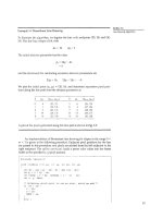
Example
3-1
Bresenham Line Drawing
~ine-Drawing Algorithms
To illustrate the algorithm, we digitize the line with endpoints
(20, 10)
and
(30,
18).
This line has a slope of
0.8,
with
The initial decision parameter has the value
and the increments for calculating successive decision parameters are
We
plot the initial point
(xo, yo)
=
(20, lo),
and determine successive pixel posi-
tions along the line path from the decision parameter as
A
plot of the pixels generated along this line path is shown in
Fig.
3-9.
An implementation of Bresenham line drawing for slopes in
the
range
0

<
rn
<
1
is given in the following procedure. Endpoint pixel positions for the line
are passed to this procedure, and pixels are plotted from the left endpoint to the
right endpoint. The call to
setpixel
loads a preset color value into the frame
buffer at the specified
(x,
y)
pixel position.
void lineares (int
xa,
i:it
ya,
int
xb,
int
yb)
(
int
dx
=
abs (xa
-
xbl,
dy
=

abs
(ya
-
yb):
int
p
=
2
*
dy
-
dx;
int twoDy
=
2
'
dy,
twoDyDx
=
2
'
ldy
-
Ax);
int
x,
y,
xEnd:
/'
Determine

which
point
to
use
as
start,
which
as
end
*/
if
:xa
>
xb)
(
x
=
xb;
Y
=
yb;
xEnd
=
xa;
)
!
else
I
x
=

xa;
Y
=
ya;
xEnd
=
xb;
1
setpixel
(x,
y);
while (x
<
xEnd)
(
x++;
if
lp
<
0)
$3
+=
twoDy;
else
[
y++;
g
+=
twoDyDx;
)

setpixel
(x,
y);
1
1
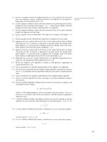
Bresenham's algorithm is generalized to lines with arbitrary slope
by
con-
sidering the symmetry between the various octants and quadrants of the
xy
plane. For a line with positive slope greater than
1,
we intelrhange the roles of
the
x
and y directions. That is, we step along they direction in unit steps and cal-
culate successive
x
values nearest the line path.
Also,
we could
revise
the pro-
gram
to plot pixels starting from either endpoint. If the initial position for a line
with
positive slope is the right endpoint, both
x
and
y

decrease as we step from
right to left. To ensure that the same pixels
are
plotted regardless of the starting
endpoint, we always choose the upper (or the lower) of the two candidate pixels
whenever the two vertical separations from the line path are equal
(d,
=
dJ.
For
negative slopes, the procedures are similar, except that now one coordinate de-
creases as the other increases. Finally, specla1 cases can
be
handled separately:
Horizontal lines (Ay
=
01,
vertical lines
(Ar
=
O),
and diagonal lines with
I
Ar
1
=
I
Ay
1
each can

be
loaded directly into the frame buffer without processing them
through the line-plotting algorithm.
Parallel
Line
Algorithms
The line-generating algorithms we have discussed
so
far determine
pixel
posi-
tions sequentially. With a parallel computer, we can calculate pixel positions
Figure
3-9
Pixel
positions along the line path
between
endpoints
(20.10)
and
(30,18),
plotted with Bresenham's
hne algorithm.
along a line path simultaneously by partitioning the computations among the
Wion3-2
various processors available. One approach to the partitioning problem is to
Line-Drawing
~lgorithms
adapt an existing sequential algorithm to take advantage of multiple processors.
Alternatively, we

can
look for other ways to set
up
the processing
so
that pixel
positions can be calculated efficiently in parallel.
An
important consideration in
devising a parallel algorithm
is
to balance the processing load among the avail-
able processors.
Given
n,
processors, we can set up a parallel Bresenham line algorithm by
subdividing :he line path into
n,
partitions and simultaneously generating line
segments in each of the subintervals. For a line with slope
0
<
rn
<
I
and left
endpoint coordinate position
(x,
yo),
we partition the line along the positive

x
di-
rection. The distance between beginning
x
positions of adjacent partitions can
be
calculated as
where Ax
is
the width of the line, and the value
for
partition width
Ax.
is
com-
puted using integer division. Numbering the partitiois, and the as
0,
1,2,
up to n,
-
1,
we calculate the starting
x
coordinate for the kth partition as
As
an example, suppose Ax
=
15
and we have np
=

4
processors. Then the width
of the partitions is
4
and the starting
x
values for the partitions are xo,
xo
+
4,
x,
+
8,
and x,
+
12.
With this partitioning scheme, the width of the last (rightmost)
subintewal will be smaller than the others in some cases. In addition, if the line
endpoints are not ~ntegers, truncation errors can result in variable width parti-
tions along the length of the line.
To apply Bresenham's algorithm over the partitions, we
need
the initial
value for the
y
coordinate and the initial value for the decision parameter
in
each
partition. The change
Ay,

in they direction over each partition
is
calculated from
the line slope
rn
and partition width Ax+
Ay,
=
mAxP
(3-1
7i
At the kth partition, the starting
y
coordinate is then
The initial decision parameter for Bresenl:prn's algorithm at the start of the
kth
subinterval is obtained from
Eq.
3-12:
Each processor then calculates pixel positions over its assigned subinterval using
the starting decision parameter value for that subinterval and the starting coordi-
nates
(xb
yJ. We can also reduce the floating-point calculations to integer arith-
metic in the computations for starting values yk and
pk
by substituting
m
=
Ay/Ax and rearranging terms. The extension of the parallel Bresenham algorithm

to a line with slope greater than
1
is achieved by partitioning the line in the
y
di-
rection and calculating beginning
x
values for the partitions. For negative slopes,

I
;i
we increment coordinate values in one direction and decrement in the other.
Another way to set up parallel algorithms on raster systems is to assign
each pmessor to
a
particular group of screen pixels. With a sufficient number of
processors (such as a Connection Machine CM-2 with over
65,000
processors), we
can assign each processor to one pixel within some screen region.
Thii
approach
I
I
v1
J
can be adapted to line display by assigning one processor to each of the pixels
-AX-
Whin the limits of the line coordinate extents (bounding rectangle) and calculating
pixel distances from the line path. The number of pixels within the bounding box

of a line is
Ax.
Ay
(Fig.
3-10).
Perpendicular distance
d
from the line in Fig.
3-10
to
Xl
a pixel with coordinates
(x,
y)
is obtained with the calculation
Figure
3-10
d=Ax+By+C
(3-20)
Bounding
box for a
Line
with
coordinate extents
band
Ay.
where
A=
-A~,
linelength

Ax
B
=
linelength
with
linelength
=
Once the constants
A,
B,
and
C
have been evaluated for the line, each processor
needs to perform two multiplications and two additions to compute the pixel
distanced. A pixel is plotted if d is less than a specified line-thickness parameter.
lnstead of partitioning the screen into single pixels; we can assign to each
processor either a scan line or a column of pixels depending on the line slope.
Each processor then calculates the intersection of the line with the horizontal row
or vertical column of pixels assigned that processor. For
a
line with slope
1
m
I
<
1,
each processor simply solves the line equation for
y,
given an
x

column value.
For a line with slope magnitude greater than
1,
the line equation is solved for
x
by each processor, given a scan-line
y
value. Such direct methods, although slow
on sequential machines, can be performed very efficiently using multiple proces-
SOTS.
3-3
LOADING
THE
FRAME
BUFFER
When straight line segments and other objects are scan converted for display
with a raster system, frame-buffer positions must be calculated. We have as-
sumed that this is accomplished with the
setpixel
procedure, which stores in-
tensity values for the pixels at corresponding addresses within the frame-buffer
array. Scan-conversion algorithms generate pixel positions at successive unit in-
-
-

-
.
.
-
-

Fiprr
3-1
I
Pixel screen pos~t~ons stored linearly in row-major order withm the
frame
buffer.
tervals. This allows us to use incremental methods to calculate frame-buffer ad-
dresses.
As a specific example, suppose the frame-bulfer array is addressed in row-
major order and that pixel positions vary from
(0.
0)
at the lower left screen cor-
ner to (x,,
y,,,)
at the top right corner (Fig.
3-11).
For a bilevel system
(1
bit per
pixel), the frame-buffer bit address for pixel position (x, y)
is
calculated as
Moving across a scan line, we can calculate the frame-buffer address for the pixel
at
(X
+
1,
y) as the following offset from the address for position (x, y):

Stepping diagonally up to the next scan line
from
(x,
y),
we get to the frame-
buffer address of
(x
+
1,
y +
1) with the calculation
addr(x
+
1,
y
+
1)
=
addr(x,
yl
+
x,,,
-1-
2
(3-23)
where the constant x,,,
+
2
is precomputed once for all line segments. Similar in-
cremental calculations can be obtained fmm Eq. 3-21 for unit steps in the nega-

tive x and
y
screen directions. Each of these address calculations involves only a
single integer addition.
Methods for implementing the
setpixel
procedure to store pixel intensity
values depend on the capabilities of a particular system and the design require-
ments of the software package. With systems that
can
display a range of intensity
values for each pixel, frame-buffer address calculations would include pixel
width (number of bits), as well as the pixel screen location.
3-4
LINE FUNCTION
A procedure for specifying straight-line segments can be set up in a number of
different forms. In
PHIGS,
GKS,
and some other packages, the two-dimensional
line function is
Chapter
3
polyline (n, wcpoints)
Output
Primit~ves
where parameter
n
is
assigned an integer value equal to the number of coordi-

nate positions to
be
input, and
wcpoints
is the array of input worldcoordinate
values for line segment endpoints. This function is used to define a set of
n
-
1
connected straight line segments. Because series of connected line segments
occur more often than isolated line segments in graphics applications,
polyline
provides a more general line function. To display a single shaight-line segment,
we set
n
-=
2
and list the
x
and
y
values of the two endpoint coordinates in
As an example of the use of
polyline,
the following statements generate
two connected line segments, with endpoints at
(50,
103, (150,
2501,
and

(250,
100):
wcPoints[ll .x
=
SO;
wcPoints[ll .y
=
100;
wcPoints[21 .x
=
150;
wc~oints[2l.y
=
250;
wc~oints[3l.x
=
250;
wcPoints[31
.y
=
100;
polyline
(3,
wcpoints);
Coordinate references in the
polyline
function are stated as absolute coordi-
nate values.
This
means that the values specified are the actual point positions in

the coordinate system
in
use.
Some
systems employ line (and point) functions with relative co-
ordinate
specifications.
In this case, coordinate values are stated as offsets
from
the last position referenced (called the current position). For example, if location
(3,2)
is the last position that has been referenced in an application program, a rel-
ative coordinate specification of
(2,
-1)
corresponds to an absolute position of
(5,
1). An additional function
is
also available for setting the current position before
the line routine
is
summoned. With these packages,
a
user lists only the single
pair of offsets
in
the line command. This signals the system to display a line start-
ing from the current position to a final position determined by the offsets. The
current posihon

is
then updated to this final line position. A series of connected
lines is produced with such packages by a sequence of line commands, one for
each line section to
be
drawn. Some graphics packages provide options allowing
the user to
specify
Line endpoints using either relative or absolute coordinates.
Implementation of the
polyline
procedure is accomplished by first per-
forming a series of coordinate transformations, then
malung
a sequence of calls
to a device-level line-drawing routine. In
PHIGS,
the input line endpoints are ac-
tually specdied in modeling coordinates, which are then converted to world
ce
ordinates. Next, world coordinates are converted to normalized coordinates, then
to device coordinates. We discuss the details for carrying out these twodimen-
sional coordinate transformations in Chapter
6.
Once in device coordinates, we
display the plyline by invoking
a
line routine, such as Bresenham's algorithm,
n
-

1
times
to connect the
n
coordinate points. Each successive call passes the
cc~
ordinate pair needed to plot the next line section, where the first endpoint of each
coordinate pair is the last endpoint of the previous section. To avoid setting the
intensity of some endpoints twice, we could
modify
the
line
algorithm so that the
last endpoint of each segment
is
not plotted.
We
discuss methods for avoiding
overlap of displayed objects in more detail in Section
3-10.
3-5
CIRCLE-GENERATING ALGORITHMS
Since
the circle is a frequently used component in pictures and graphs, a proce-
dure for generating either
full
circles or circular arcs
is
included in most graphics
packages. More generally,

a
single procedure can
be
provided to display either
circular or elliptical
curves.
Properties of Circles
A
ckle is defined as the set of points that are
all
at a given distance
r
from
a cen-
ter position (x,,
y,)
(Fig.
3-12).
This
distance relationship is expressed by the
Pythagorean theorem in Cartesian coordinates as
We could use this equation to calculate the position of
points
on a ciicle circum-
ference by stepping along the x axis
in
unit steps from x,
-
r
to x,

+
r
and calcu-
lating the corresponding y values at each position as
But this
is
not the best method for generating a circle.
One
problem with this ap
proach is that it involves considerable computation at each step. Moreover, the
spacing between plotted pixel positions
is
not uniform,
as
demonstrated in Fig.
3-13.
We
could adjust the spacing by interchanging
x
and
y
(stepping through
y
values and calculating x values) whenever the absolute value of the slope of the
circle is greater than
1.
But this simply increases the computation and processing
required
by
the

algorithm.
Another way to eliminate the unequal spacing shown in Fig.
3-13
is to cal-
culate points along the circular boundary using polar coordinates r and
8
(Fig.
3-12).
Expressing the circle equation in parametric polar form yields the pair of
equations
When
a display is generated with these equations using a fixed angular step size,
a
circle is plotted with equally spaced points along the circumference. The step
size chosen for
8
depends on the application and the display device. Larger an-
gular separations along the circumference can be connected with straight line
segments to approximate the circular path. For a more continuous boundary on a
raster display, we can set the step size at
l/r.
This plots pixel positions that are
approximately one unit apart.
Computation can
be
reduced by considering the symmetry of circles. The
shape of the circle is similar in each quadrant. We can generate the circle section
in (he second quadrant of the
xy
plaie by noting that the two circle sections are

symmetric with respect to they axis. And circle sections in the third and fourth
Figure
3-12
Circle with center
coordinates
(x,,
y,)
and radius r.
Figure
3-13
Positive
half of
a
circle
plotted with
Eq.
3-25
and
with
(x,,
y,)
=
(0.0).
quadrants can
be
obtained
from
sections in the first and second quadrants by
Y
I

considering symmetry about the
x
axis. We can take this one step further and
-
-
note that there
is
alsd symmetry between octants. Circle sections in adjacent
oc-
tants within one quadrant are symmetric with respect to the 45' line dividing the
two octants. These symmehy conditions are illustrated in Fig.3-14, where a point
at position
(x,
y) on a one-eighth circle sector is mapped into the seven circle
points in the other octants of the
xy
plane. Taking advantage of the circle symme-
try
in this way we can generate all pixel positions around a circle by calculating
only the points within the sector from
x
=
0
to
x
=
y.
Determining pixel positions along a circle circumference using either Eq.
3-24
or Eq.

3-26
still requires a
good
deal of computation time. The Cartesian
I
equation 3-24 involves multiplications and squar&oot calculations, while the

parametric equations contain multiplications and trigonometric calculations.
Figure
3-14
More efficient circle algorithms are based on incremental calculation of decision
Symmetry of
a
circle.
-parameters, as in the Bresenham line algorithm, which mvolves only simple inte-
Calculation
of
a circle point
ger
operations,
(I,
y)
in one &ant yields the
Bresenham's line algorithm for raster displays is adapted to circle genera-
circle points shown for the
tion by setting up decision parameters for finding the closest pixel to the circum-
other seven octants.
ference at each sampling step. The circle equation
3-24,
however, is nonlinear, so

that squaremot evaluations would
be
required to compute pixel distances from a
circular path. Bresenham's circle algorithm avoids these square-mot calculations
by comparing the squares of the pixel separation distances.
A method for direct distance comparison is to test the halfway position be
tween two pixels to determine if this midpoint is inside or outside the circle
boundary.
This
method is more easily applied to other conics; and for an integer
circle radius, the midpoint approach generates the same pixel positions as the
Bresenham circle algorithm. Also, the error involved in locating pixel positions
along any conic section using the midpoint test is limited to one-half the pixel
separation.
Midpoint Circle Algorithm
As in the raster line algorithm, we sample at unit intervals and determine the
closest pixel position to the specified circle path at each step. For a given radius
r
and screen center position
(x,
y,), we can first set up our algorithm to calculate
pixel positions around a circle path centered at the coordinate origin
(0,O).
Then
each calculated position
(x,
y) is moved to its proper screen position by adding
x,
to
x

and
y,
toy. Along the circle section from
x
=
0
to
x
=
y in the first quadrant,
the slope of the curve varies from
0
to
-1.
Therefore, we can take unit steps in
the positive
x
direction over this octant and use a decision parameter to deter-
mine which of the two possible y positions
is
closer to the circle path at each step.
Positions ih the other seven octants are then obtained by symmetry.
To apply the midpoint method, we define a circle function:
Any point
(x,
y)
on the boundary of the circle with radius
r
satisfies the equation
/cin,,(x,

y)
=
0.
If the point is in the interior of the circle, the circle function is nega-
tive. And if the point is outside the circle, the circle function is positive.
To
sum-
marize, the relative position of any point
(x.
v)
can be determined by checking the
sign of the circle function:
f
<
0,
if
(x,
V)
is inside the drde boundary
Ill1
-
-"
if
(x,
y)
is
on the circle boundary
xz
+
yt

-
rz
-0
>
0,
if
(x,
y)
is
outside the circle boundary
The circle-function tests in
3-28
are
performed
for the midpositions between pix-
els near the circle path at each sampling step.
Thus,
the circle function
is
the deci-
xk
x,
+
1
x,
+
2
sion parameter in the midpoint algorithm, and we can set up incremental calcu-
lations for this function as we did in the line algorithm.
'

Figure 3-15 shows the midpoint between the two candidate pixels
at
Sam-
Figrrre3-15
pling position
xk
+
1.
Assuming we have just plotted the pixel at (xk,
yk),
we next
Midpoint
between
candidate
pixels
at
sampling
position
nd
to determine whether the pixel at position
(xk
+
1,
yk)
or the one at position
xk+l
cirrular
path.
(xk
+

1,
yk

1)
is
closer to
the
circle.
Our
decision parameter is the circle function
3-27
evaluated at the midpoint between these two pixels:
If
pk
<
0,
this midpoirat is inside the circle and the pixel on scan line
yb
is
closer to
the circle boundary. Otherwise, the midposition is outside or on the circle bound-
ary, and we select the pixel on scanline
yk
-
1.
Successive decision parameters are obtained using incremental calculations.
We obtain a recursive expression for the next decision parameter by evaluating
the circle function at sampling p~sitionx~,,
+
1

=
x,
+
2:
where
yk
,,
is either
yi
or
yk-,,
depending on the sign of
pk.
increments
for obtaining
pk+,
are either
2r,+,
+
1
(if
pk
is
negative) or
2r,+,
+
1
-
2yk+l.
Evaluation of the terms

Zk+,
and
2yk+,
can also
be
done inaemen-
tally as
At the start position
(0, T),
these two terms have the values
0
and
2r,
respectively.
Each successive value is obtained by adding
2
to the previous value of
2x
and
subtracting
2
from the previous value of
5.
The initial decision parameter is obtained by evaluating the circle function
at the start position
(x0,
yo)
=
(0,
T):

Chaw
3
Output
Primitives
5
pO=cr
(3-31)
If
the radius
r
is
specified
as
an
integer,
we
can
simply round
po
to
po
=
1
-
r
(for
r
an
integer)
since

all
inmments
are
integers.
As
in Bresenham's line algorithm, the midpoint method calculates pixel
po-
sitions along the circumference of a cirde using integer additions and subtrac-
tions,
assuming that the circle parameters
are
specified in integer screen
coordi-
nates.
We can summarize the steps in the midpoint circle algorithm as follows.
Midpoint
Circle
Algorithm
1.
hput radius
r
and circle center (x, y,), and obtain the first point on
the
circumference
of
a
circle centered on the origin as
I
2.
cdculate the initial value

of
the decision parameter as
3.
At
each xk
position,
starting at
k
=
0,
perform the following test: If
pk
C
0,
the next
point
along the circle centered on
(0,O)
is
(xk,,, yk) and
I
Otherwise,
the
next point along the circle
is
(xk
+
1,
yk
-

1)
and
where 2xk+,
=
kt
+
2
and
2yt+,
=
2yt
-
2.
4.
~eterrnine symmetry
points
in the other seven octants.
5.
Move each calculated pixel
position
(x, y) onto the
cirmlar
path cen-
tered
on
(x,
yc)
and
plot the coordinate values:
x=x+xc, y=y+yc

6.
Repeat steps
3
through
5
until
x
r
y.
Section
3-5
C
ircle-Generating Algorithms

Figure
3-16
Selected pixel positions (solid
circles)
along a circle path with
radius
r
=
10
centered on
the
origin,
using the midpoint circle algorithm.
Open
circles show the symmetry
positions

in
the first quadrant.
Example
3-2
Midpoint Circle-Drawing
Given a circle radius
r
=
10, we demonstrate the midpolnt circle algorithm
by
determining positions along the circle octant in the first quadrant hum
x
=
0 to
x
=
y.
The initial value of the decision parameter is
For the circle centered on the coordinate origin, the initial point is
(x,,
yo)
-
(0,
lo), and initial increment terms for calculating the dxision parameters are
Successive decision parameter values and positions along the circle path are cal-
culated using the midpoint method as
A
plot
c
)f

the generated pixel positions in the first quadrant is shown in Fig.
3-10.
The
following procedure displays a raster tide on a bilevel monitor using
the midpoint algorithm. Input to the procedure are the coordinates for the circle
center and the radius. Intensities for pixel positions along the circle circumfer-
ence are loaded into the frame-buffer array with calls to the
set
pixel
routine.
Chapter
3
Ouipur
Pr~mitives
Figure
3-1
7
Ellipse
generated
about
foci
F,
and
F,.
#include 'device
.h
void circleMidpoint (int Kenter, int yCenter, int radius)
I
int x
=

0;
int
y
=
radius;
int
p
=
1
-
radius;
void circlePlotPoints (int, int, int, int);
/'
Plot first set
of
points
'/
circlePlotPoints (xcenter. *enter. x,
yl;
while (x
<
y)
(
x++
;
if
(P
<
O!
+

p
*=
2
else
I
Y ;
p
+z
2
'
(x
-
Y)
+
1;
void circlePlotPolnts (int xCenter, int yCenter, int
x,
int
yl
(
setpixel (xCenter
+
x, $enter
+ y);
setpixel (xCenter
-
x. $enter
+
yl;
setpixel (xCenter

+
x,
$enter
-
y);
setpixel (xCenter
-
x,
$enter
-
y);
setpixel (xCenter
+
y,
$enter
+
x);
setpixel
(xCenter
-
y,
$enter
+
x);
setpixel (xCenter
t
y,
$enter
-
x);

setpixel
(xCenter
-
y,
$enter
-
x);
1
3-6
ELLIPSE-GENERATING ALGORITHMS
Loosely
stated,
an ellipse
is
an elongated circle. Therefore, elliptical
curves
can
be
generated
by
modifying
circle-drawing
procedures
to take into account the dif-
ferent dimensions of an ellipse along the mapr and minor axes.
Properties
of
Ellipses
An
ellipse

is
defined as the set
of
points such that the sum of the distances
from
two
fi.ted
positions (foci)
is
the
same
for
all
points
(Fig.
b17).
Lf
the distances to
the two
foci from
any point
P
=
(x,
y)
on the ellipse are labeled
dl
and
d2,
then the

general equation of an ellipse can
be
stated as
d,
+
d,
=
constant
(3-321
Expressing
distances
d,
and
d,
in
terms of
the
focal coordinates
F,
=
(x,,
y,)
and
F2
=
(x,
y2),
we
have
By squaring this equation, isolating the remaining radical, and then squaring

again, we can rewrite the general ellipseequation in the
form
Ax2
+
By2
+
Cxy
+
Dx
+
Ey
+
F
=
0
(3-34)
where the coefficients
A,
B,
C,
D,
E,
and Fare evaluatcul in terms of the focal coor-
dinates and the dimensions of the major and minor axes of the ellipse. The major
axis is the straight line segment extending from one side of the ellipse to the
other through the foci. The minor axis spans the shorter dimension of the ellipse,
bisecting the major axis at the halfway position (ellipse center) between the two
foci.
An interactive method for specifying an ellipse in an arbitrary orientation is
to input the two foci and a point on the ellipse boundary. With these three coordi-

nate positions, we can evaluate the constant in Eq.
3.33.
Then, the coefficients in
Eq.
3-34 can be evaluated and used to generate pixels along the elliptical path.
Ellipse equations are greatly simplified
if
the major and minor axes are ori-
ented to align with the coordinate axes. In Fig. 3-18, we show an ellipse in "stan-
ddrd position" with major and minor axes oriented parallel to the
x
and
y
axes.
Parameter
r,
for this example labels the semimajor axis, and parameter
r,,
labels
the semiminor axls. The equation of the ellipse shown in Fig. 3-18 can be written
in terms of the ellipse center coordinatesand parameters
r,
and
r,
as
Using
polar coordinates
r
and
0.

we can also describe the ellipse
in
standard posi-
tion with the parametric equations:
T
=
x,.
t
r,
cosO
y
=
y,.
+
r,
sin9
Symmetry considerations can be used to further reduce con~putations. An ellipse
in stdndard position is symmetric between quadrants, but unlike a circle, it is not
synimrtric between the two octants of a quadrant. Thus, we must calculate pixel
positions along the elliptical arc throughout one quadrant, then we obtain posi-
tions in the remaming three quadrants by symmetry (Fig 3-19).
Our approach hrrr is similar
to
that used in displaying
d
raster circle. Given pa-
rameters
r,,
r!,
a~ld

(x,,
y,.),
we determine points
(x,
y)
for an ellipse in standard
position centered on the origin, and then we shift the points so the ellipse
is
cen-
tered at
(x,
y,).
1t
we
wish also tu display the ellipse in nonstandard position, we
could then rotate the ellipse about its center coordinates to reorient the major and
minor
axes. For
the
present,
we
consider only the display of ellipses in standard
position
We
discuss general methods for transforming object orientations and
positions in Chapter
5.
The
midpotnt ellipse niethtd is applied throughout thc first quadrant in
t\co parts. Fipurv

3-20
shows the division of the first quadrant according to the
slept,
of
an
ellipse with
r,
<
r,.
We process this quadrant by taking unit steps
in
the
.j
directwn where the slope of the curve has a magnitude less than
1,
and tak-
ing unit steps in thcy direction where the slop has
a
magnitude greater than
1.
Regions
I
and
2
(Fig.
3-20),
can he processed in various ways. We can start
at position
(0.
r,)

c*nd step clockwise along the elliptical path in the first quadrant,
.


Figure
3-18
Ellipse
centered at
(x,,
y,)
with
wmimajor axis
r,
and
st:miminor axis
r,.
Clldprer
3
shlfting from unit steps in
x
to unit steps in
y
when the slope becomes less than
~utpul Pr~rnitives
-1.
Alternatively, we could start at
(r,,
0)
and select points in a countexlockwise
order, shifting from unit steps in

y
to unit steps in
x
when the slope becomes
greater than
-1.
With parallel processors, we could calculate pixel positions in
the two regions simultaneously. As an example of a sequential implementation of
(-x.
v)
(,
y,
the midpoint algorithm, we take the start position at
(0,
ry)
and step along the el-
&
lipse path in clockwise order throughout the first quadrant.
We define an ellipse function from
Eq.
3-35
with
(x,,
y,)
=
(0,O)
as
-
I-
x.

-
yl
(X
-y)
which has the following properties:
1
0,
if
(x,
y)
is
inside the ellipse boundary
Symmetry
oi
an cll~pse
>
0
if
(x,
y)
is outside the ellipse boundary
Calculation
IJ~
a
pint
(x,
y)
In
one quadrant yields
the

Thus,
the ellipse function
f&,(x,
y)
serves as the decision parameter in the
mid-
ell'pse points
shown
for
the
point algorithm. At each sampling position, we select the next pixel along the el-
other three quad rants.
lipse
path according to the sign of the ellipse function evaluated at the midpoint
between
the two candidate pixels.
v
t
Starting at
(0,
r,),
we take unit steps
in
the
x
direction until we reach the
boundary between region
1
and region 2-(~i~.
3-20).

Then we switch to unit steps
in the
y
direction over the remainder
of
the curve in the first quadrant. At each
step, we need to test the value of the slope of the curve. The ellipse slope is calcu-
lated
from
Eq.
3-37
as

1
At the boundary between region
1
and region
2,
dy/dx
=
-
1
and
-
-
-
-
.
-
-

.
.
-
.
-
-
-
F~,y~rn'
3-20
Ellipse processing regions.
Over
regior
I,
the magnitude
of
the ellipse slope
is
less
than
1;
over region
2,
the
magnitude
of
the slope is
greater than
I.
Therefore, we move out of region

1
whenever
Figure
3-21
shows the midpoint between the two candidate pixels at
sam-
piing position
xk
+
1
in the first regon. Assuming position
(xk,
yk)
has been
se-
lected at the previous step,
we
determine the next position along the ellipse path
by evaluating the decision parameter (that is, the ellipse function
3-37)
at this
midpoint:
If
pl,
<
0,
the midpoint is inside the ellipse and the pixel on scan line
y,
is
closer

to the ellipse boundary. Otherwise, the midposition is outside or on the ellipse
boundary, and we
select
the pixel on scan line
yt
-
1.
At the next sampling position
(xk+,
+
1
=
x,
+
2),
the decision parameter
for region
1
is evaluated as
Yt
p1i+l
=
feUip(xk+l
+
yk+,
-
i)
v,
-
1

(
-
f)'-r:rt
=
r;[(xk
+
1)
+
112
+
T:
Yk+,
x,
X,
+
1
l2
M';dpoint between candidate
plk+, =~1~+2r;(xk+l)+ri +r;[(yk+r
k)27(yk-
(M2)
pixels
at sampling position
xl
+
1
along an elliptical
path.
where
yk+,

is either
yl,
or
yk
-
1,
depending on the sign of
pl,.
Decision parameters are incremented by the following amounts:
2r,?~k+~
+
r:,
if
plk
<
0
increment
=
2
+
r
-
2
if
plk
2
0
As in the circle algorithm, increments for ihe decision parameters can be calcu-
lated using only addition and subtraction, since values for the terms
2r;x

and
2r:y
can also
be
obtained incrementally. At the initial position
(0,
r,),
the two
terms evaluate to
As
x
and
y
are incremented, updated values are obtained by adding
2ri
to
3-43
and subtracting
21:
from
3-44.
The
updated values are compared at each step,
and we move from region
1
to region
2
when condition
3-40
is satisfied.

Jn region
1,
the initial value of the decision parameter is obtained
by
evalu-
ating the ellipse function at the start position
(x, yo)
=:
(0,
r,):
1
pl,
=
r,?
-
r;ry
+
-
r,2
4
(3-45)
Over region
2,
we sample at unit steps in the negative
y
direction, and the
midpoint is now taken between horizontal pixels
at
each step (Fig.
3-22).

For this
region, the decision parameter is evaJuated as
Chaoter
3
Oufput
Primitives
Figlrrc
3-22
Midpoint between candidate pixels
at
sampling
position
y,
-
1
along an
x,
x,
+
1
x,
+
2
elliptical path.
If
p2,
>
0,
the midposition is outside the ellipse boundary, and we select the pixel
at

xk.
If
pa
5
0,
the midpoint is inside or on the ellipse boundary, and we select
pixel position
x,,
,.
To determine the relationship between successive decision parameters in
region
2,
we evaluate the ellipse function at the next sampling step
yi+,
-
1
-
y~
-
2:
with
xk
+
,
set
either
to
x,
or to
xk

+
I,
depending on the sign
of
~2~.
When we enter region
2,
;he initial position
(xo,
yJ
is taken as the last
posi-
tion selected in region
1
and the initial derision parameter in region
2
is then
To
simplify the calculation of
p&,
we could select pixel positions in counterclock-
wise
order starting at
(r,,
0). Unit steps would then
be
taken in the positive
y
di-
rection up to the last position selected in rrgion

1.
The
midpoint algorithm can
be
adapted to generate an ellipse in nonstan-
dard position using the ellipse function
Eq.
3-34
and calculating pixel positions
over the entire elliptical path. Alternatively, we could reorient the ellipse axes to
standard position, using transformation methods discussed in Chapter
5,
apply
the midpoint algorithm to determine curve positions, then convert calculated
pixel positions to path positions along the original ellipse orientation.
Assuming
r,,
r,,
and the ellipse center are given in integer screen
coordi-
nates, we only
need
incremental integer calculations to determine values for the
decision parameters in the midpoint ellipse algorithm. The increments
rl,
r:,
2r:,
and
2ri
are evaluated once at the beginning of the procedure.

A
summary of the
midpoint ellipse algorithm is listed
in
the following steps:
Midpoint Ellipse
Algorithm
1.
Input
r,,
r,,
and ellipse center
(x,,
y,), and obtain the first point on an
ellipse centered on the origin as
2.
Calculate the initial value of thedecision parameter in region 1 as
3.
At each
x,
position in region
1,
starting at
k
=
3,
perform the follow-
ing test:
If
pl,

<
0, the next point along the ellipse centered on (0,
0)
is
(x,
.
I,
yI)
and
Otherwise, the next point along the circle is
(xk
+
1,
yr,
-
1) and
with
and continue until
2rix
2
2rty.
4.
Calculate
the initial value of the decision parameter in region
2
using
the last point
(xo,
yo) calculated in region
1

as
5.
At each
yk
position in region
2,
starting at
k
=
0,
perform the follow-
ing test:
If
pZk>
0, the next point along the ellipse centered on (0, 0) is
(xk,
yk

1)
and
Otherwise, the next point along the circle
is
(.rk
+
1,
yt
-
1)
and
using the same incremental calculations for

.I
and
y
as in region
1.
6.
Determine symmetry points in the other three quadrants.
7.
Move each calculated pixel
position
(x,
y)
onto
the
elliptical
path
cen-
tered on
(x,,
y,)
and plot the coordinate values:
8.
Repeat the steps for region
1
until
26x
2
2rf.y
Ellipse-Generating Algorilhrns
Chapter

3
Oucpur
Example
3-3
Midpoint Ellipse Drawing
Given input ellipse parameters
r,
=
8
and
ry
=
6,
we illustrate the steps in the
midpoint ellipse algorithm by determining raster positions along the ellipse path
in the first quadrant. lnitial values and increments for the decision parameter cal-
culations are
2r:x
=
0
(with increment
2r;
=
72)
Zrfy=2rfry
(withincrement-2r:=-128)
For region
1:
The
initial point for the ellipse centered on the origin is

(x,,
yo)
=
(0,6),
and the initial decision parameter value
is
1
pl,
=
r;
-
rfr,
t
-
r:
=
-332
4
Successive decision parameter values and positions along the ellipse path are
cal-
culated using the midpoint method as
We
now
move
out
of region
1,
since
2r;x
>

2r:y.
For region
2,
the initial point is
(x,
yo)
=
V,3)
and the initial decision parameter
is
The remaining positions along the ellipse path in the
first
quadrant
are
then
cal-
culated as
A
plot of the selected positions around the ellipse boundary within the first
quadrant
is
shown in Fig.
3-23.
In the following procedure, the midpoint algorithm is
used
to display an el-
lipsc: with input parameters
RX,
RY, xcenter,
and

ycenter.
Positions along the
Section
36
Flltpse-Generating Algorithms
Figure
3-23
Positions along
an
elliptical path
centered on the
origin
with
r,
=
8
and
r,
=
6
using the midpoint
algorithm to calculate pixel
addresses
in
the first quadrant.
curve in the first quadrant are generated and then shifted to their proper screen
positions. Intensities
for
these positions and the symmetry positions in the other
th quadrants are loaded into the frame buffer using the

set
pixel
mutine.
void ellipseMidpoint (int xCenter, int yCenter, int
Rx,
int Ry)
(
int Rx2
=
Rx4Rx;
int RyZ
=
RygRy;
int twoRx2
=
2.Rx2;
int twoRy2
=
2*RyZ;
int
p;
int x
=
0;
int y
=
Ry;
int px
=
0;

int py
=
twoRx2 y;
void ellipsePlotPoints (int, int, int,
int);
1.
Plot
the
first
set of
points
'I
ellipsePlotPoints (xcenter, yCenter,
X,
Y);
/*
Region
1
*I
P
=
ROW
(Ry2
-
(Rx2 Ry)
+
(0.25
.
-2));
while (px

<
PY)
{
x++;
px
+=
twoxy2;
if
(p
c
0)
p
+=
Ry2
+
px;
else
(
y ;
py
-=
twoRx2;
p
+=
Ry2
+
px
-
py;
1

/*
Region 2
*/
p
=
ROUND (RyZ*(x+0.5)'(%+0.5)
+
Rx2*(y-l)'(y-l)
-
Rx2.Ry2);
while (y
>
0)
(
Y ;
py
-=
twoRx2;
if
(p
>
0)
p
+=
Rx2
-
py;
else
(
x++;

px
+=
twoRy2:
p
+=
Rx2
-
PY
+
Px;
Chanter
3
1
Output Primitives
1
e1l:poePlotFo~n:s
(xCellLr~,
ycenter,
x,
yl;
void ellipsePlotPo-nts (int xCenter, int yCenter,
int
x,
int
yl
(
setpixel (xCentel.
+
x,
yCenter

+
yl
:
setpixel (xCente1-
-
x,
yCencer
+
y);
setpixel (xCente1-
t
x, yCenter
-
y);
setpixel (xCenter
-
x,
$enter
-
y):
OTHER
CURVES
Various curve functions are useful in object modeling, animation path specifica-
tions, data and function graphing, and other graphics applications. Commonly
encountered curves include conics, trigonometric and exponential functions,
probability distributions, general polynomials, and spline functions. Displays of
these
curves
can be generated with methods similar to those discussed for the
circle and ellipse functions. We can obtain positions along curve paths directly

from explicit representations
y
=
f(x)
or from parametric forms Alternatively, we
could apply the incremental midpoint method to plot curves described with im-
plicit functions
fix,
y)
=
1).
A straightforward method for displaying a specified curve function is to ap-
proximate it with straight line segments. Parametric representations are useful in
this case for obtaining equally spaced line endpoint positions along the curve
path. We can also generate equally spaced positions from an explicit representa-
tion by choosing the independent variable according to
the
slope of the curve.
Where the slope of
y
=
,f(x) has a magnitude less than
1,
we choose
x
as the inde-
pendent variable and calculate
y
values at equal x increments. To obtain equal
spacing where the slope has a magnimde greater than

1,
we use the inverse func-
tion,
x
=
f
-'(y),
and calculate values of
x
at equal
y
steps.
Straight-line or cun7e approximations are used to graph a data set of dis-
crete coordinate points. We could join the discrete points with straight line seg-
ments, or we could use linear regression (least squares) to approximate !he data
set
with a single straight line. A nonlinear least-squares approach is used to dis-
play the data set with some approximatingfunction, usually a polynomial.
As with circles and ellipses, many functions possess symmetries that can be
exploited to reduce the computation of coordinate positions along curve paths.
For example, the normal probability distribution function is symmetric about a
center position (the mean), and all points along one cycle of a sine curve can be
generated from the points in a
90"
interval.
Conic
Sectior~s
In general, we can describe a conic section (or conic) with the second-degree
equation:
.4x2

+
By2
+
Cxy
+
Dx
+
Ey
+
F
=
0
(3
50)
where values for parameters
A,
B,
C,
D,
E,
and
F
determine the kind of curve we
section
3-7
are to display. Give11 this set of coefficients, we can dtatermine the particular conic
Other
Curves
that will be generated by evaluating the discriminant
R2

-
4AC:
[<
0,
generates an ellipse (or circle)
B2
-
41C
{
=
0,
generates a parabola
(.3-5
1
)
I>
0,
generates a hyperbola
For example, we get the circle equation
3-24
when
.4
=
B
=
1,
C
=
0,
D

=
-2x,,
E
=
-2y(,
and
F
=
x:
+
yf
-
r2.
Equation
3-50
also describes the "degenerate"
conics: points and straight lines.
Ellipses, hyperbolas, and parabolas are particulilrly useful in certain aninia-
tion applications. These curves describe orbital and other motions for objects
subjected to gravitational, electromagnetic, or nuclear forces. Planetary orbits in
the solar system, for example, are ellipses; and an object projected into-a uniform
gravitational field travels along a parabolic trajectory. Figure
3-24
shows a para-
bolic path in standard position for a gravitational field acting in the negative
y
di-
rect~on. The explicit equation for the parabolic trajectory of the object shown can
be written as
y

=
yo
+
a(x
-
x,J2
+
b(x
-
:to)
with constants
a
and
b
determined by the initial velocity
g
cf the object and the
acceleration
8
due to the uniform gravitational force. We can also describe such
parabolic motions with parametric equations using a time parameter
t,
measured
in seconds from the initial projection point:
xo
X
=
Xo
S
Grot

(3-33,
F~,~I~w
.3-24
1
I/
yo
+
v,,t
-
2
gf2
P,lrabolic path of
an
object
tossed into
a
downward
Here,
v,,
and
v,yo
are the initial velocity components, and the value of
g
near the
gravitational field at the
ir.~tial position
(x,,,
,yo).
surface of the earth is approximately 980cm/sec2. Object positions along the par-
abolic path are then calculated at selected time steps.

Hyperbolic motions (Fig.
3-25)
occur in connection with the collision of
charged particles and in certain gravitational problems. For example, comets or
meteorites moving around the sun may travel along hyperbolic paths and escape
to outer space, never to return. The particular branch (left or right,
in
Fig.
3-25)
describing the motion of an object depends on the forces involved in the prob-
lem. We can write the standard equation for the hyperbola cented on the origin
in Fig.
3-25
as
-r
(3-51)
with
x
5
-r,
for the left branch and
x
z
r,
for the right branch. Since this equa-
-
tion differs from the standard ellipse equation
3-35
only in the sign between the
FIKllrr

3-25
x2
and
y2
terms, we can generate points along a hyperbolic path with a slightly
~~f~
and branches
of
a
modified ellipse algorithm. We will return to the discussion of animation applica-
hyperbola in standard
tions and methods in more detail in Chapter 16.
And
in Chapter 10, we discuss
position with symmetry axis
applications of computer graphics in scientific visuali~ation. along the
x
axis.
111
Chapter
3
Parabolas and hyperbolas possess a symmetry axis. For example, the
Ou~pu~
Prirnit~ves
parabola described by
Eq.
3-53
is
symmetric about the axis:
The methods used in the midpoint ellipse algorithm can be directly applied to

obtain points along one side of the symmetry axis of hyperbolic and parabolic
paths in the two regions:
(1)
where the magnitude of the curve slope is less than
1,
and
(2)
where the magnitude of the slope is greater than
1.
To do this, we first
select the appropriate form of Eq.
3-50
and then use the selected function to set
up expressions for the decision parameters in the two regions.
Polynomials dnd Spline Curves
A
polynomial function of nth degree in
x
is
defined as
where
n
is
a
nonnegative integer and the
a,
are constants, with
a.
Z
0.

We get a
quadratic when
n
=
2;
a cubic polynomial when
n
=
3;
a quartic when
n
=
4;
and
so forth. And we have a straight line when
n
=
1.
Polynomials are useful in a
number of graphics applications, including the design of object shapes, the speci-
fication of animation paths, and the graphing of data trends in a discrete set of
data points.
Designing object shapes or motion paths is typically done by specifying a
few points to define the general curve contour, then fitting.the selected points
with a polynomial. One way to accomplish the curve fitting is to construct a
cubic polynomial curve section between each pair of specified points. Each curve
section is then
described
in parametric form as
/

y
=
a,,,
+
a,,u
+
a,,u2
+
a,,u3
(3-57)
f '
where parameter
u
varies over the interval
0
to
1.
Values for the coefficients of
u
in
the parametric equations are determined from boundary conditions on the
curve &ions. One boundary condition is that two adjacent curve sections have
Figure
3-26
the same coordinate position at the boundary, and a second condition
is
to match
A
spline
curve

formed
with
the two curve slopes at the boundary so that we obtain one continuous, smooth
individual
cubic
curve (Fig.
3-26).
Continuous curves that are formed with polynomial pieces are
sections between specified
called spline curves, or simply splines. There are other ways to set up spline
coordinate points. curves, and the various spline-generating methods are explored in Chapter
10.
3-8
-
PARALLEL
CURVE
ALGORITHMS
Methods for exploiting parallelism in curve generation are similar to those used
in displaying straight line segments. We can either adapt a sequential algorithm
by
allocating processors according to cune partitions, or we could devise other
methods and assign processors to screen partitions.
A
parallel midpoint method for displaying circles is to divide the circular
arc from
90"
to
45c
into equal subarcs and assign a separate processor to each
subarc. As in the parallel Bresenham line algorithm, we then need to set up com-

putations to determine the beginning
y
value and decisicn parameter
pk
value for
each processor. Pixel positions are then calculated throughout each subarc, and
positions in the other circle octants are then obtained by symmetry. Similarly,
a
parallel ellipse midpoint method divides the elliptical arc over the
first
quadrant
into equal subarcs and parcels these out to separate processors. Pixel positions in
the other quadrants are determined by symmetry.
A
screen-partitioning scheme
for circles and ellipses
is
to assign each scan line crossing the curve to a separate
processor. In this case, each processor uses the circle or ellipse equation to calcu-
late curve-intersection coordinates.
For the display of elliptical am or other curves, we can simply use the scan-
line partitioning method. Each processor uses the curve equation to locate the in-
tersection positions along its assigned scan line. With processors assigned to indi-
vidual pixels, each processor would calculate the distance (or distance squared)
from the curve to its assigned pixel. If the calculated distance is less than a prede-
fined value, the pixel is plotted.
3-9
CURVE FUNCTIONS
Routines for circles, splines, and other commonly
used

curves are included in
many graphics packages. The PHIGS standard does not provide explicit func-
tions for these curves, but it does include the following general curve function:
generalizedDrawingPrimitive
In,
wc~oints, id, datalist)
where wcpoints is a list of n coordinate positions, data1
ist
contains noncoor-
dinate data values, and parameter id selects the desired function. At a particular
installation, a circle might be referenced with
id
=
1,
an ellipse with id
=
2,
and
SO
on.
As an example of the definition of curves through this PHIGS function, a
circle
(id
=
1,
say) could
be
specified by assigning the two center coordinate val-
ues to wcpoints and assigning the radius value to datalist. The generalized
drawing primitive would then reference the appropriate algorithm, such

as
the
midpoint method, to generate the circle. With interactive input, a circle could
be
defined with two coordinate
points:
the center position and a point on the cir-
cumference. Similarly, interactive specification of an ellipse can be done with
three
points: the two foci and a point on the ellipse boundary, all stod
in
wc-
points. For an ellipse in standard position,
wcpoints
could
be
assigned only the
center coordinates, with
daZalist
assigned the values for
r,
and
r,.
Splines defined
with control points would
be
generated by assigning the control point coordi-
nates to wcpoints.
Functions to generate circles and ellipses often include the capability of
drawing curve sections by speclfylng parameters for the line endpoints. Expand-

ing the parameter list allows
specification
of the beginning and ending angular
values for an arc,
as
illustrated in Fig.
3-27.
Another method for designating a cir-
Section
3-9
Curve
Functions
Figure
3-27
Circular
arc
specified
by
beginning and ending angles.
Circle center
is
at
the
coordinate origin.
Chapter
3
cular or elliptical arc
is
to input the beginning and ending coordinate positions of
Output Prim~t~ves the arc.

Figure
3-28
Lower-left section of the
screen grid referencing
Integer coord~nate positions.
Figure
0-29
Line path for a series
oi
connected line segments
between screen grid
coordinate positions.
Figure
3-30
lllum~nated pixel
a1
raster
position
(4,5).
114
PIXEL
ADDRESSING AND
OBJECT
GEOMETRY
So
far we have assumed that all input positions were given in terms of scan-line
number and pixel-posihon number across the scan line. As we saw in Chapter
2,
there are, in general, several coordinate references associated with the specifica-
tion and generation of a picture. Object descriptions are given in a world-

reference frame, chosen to suit a particular application, and input world coordi-
nates are ultimately converted to screen display positions. World descriptions of
objects are given in terms of precise coordinate positions, which are infinitesi-
mally small mathematical points. Pixel coordinates, however, reference finite
screen areas.
If
we want to preserve the specified geometry of world objects, we
need to compensate for the mapping of mathematical input points to finite pixel
areas. One way to do this is simply to adjust the dimensions of displayed objects
to account for the amount of overlap of pixel areas with the object boundaries.
Another approach is to map world coordinates onto screen positions between
pixels, so that we align object boundaries with pixel boundaries instead of pixel
centers.
Screen Grid Coordinates
An alternative to addressing display posit~ons in terms of pixel centers is to refer-
ence screen coordinates with respect to the grid of horizontal and vertical pixel
boundary lines spaced one unit apart (Fig.
3-28).
A
screen soordinale position is
then the pair of integer values identifying a grid interswtion position between
two pixels. For example, the mathematical line path for a polyline with screen
endpoints
(0,
O),
(5,2),
and (1,4) is shown in Fig.
3-29.
With the coordinate origin at the lower left of the screen, each pixel area can
be

referenced by the mteger grid coordinates of its lower left corner. Figure
3-30
illustrates this convention for an
8
by
8
section of a raster, w~th a single illumi-
nated pixel at screen coordinate position (4,
5).
In
general, we identify the area
occupied by a pixel with screen coordinates (x,
y)
as the unit square with diago-
nally opposite corners at
(x,
y)
and (x
+
1,
y
+
1). This pixel-addressing scheme
has several advantages:
It
avoids half-integer pixel boundaries, it facilitates pre-
ase object representations, and it simplifies the processing involved in many
scan-conversion algorithms and in other raster procedures.
The algorithms for line drawing and curve generation discussed in the pre-
ceding sections are still valid when applied to input positions expressed as screen

grid coordinates. Decision parameters in these algorithms are now simply a mea-
sure of screen grid separation differences, rather than separation differences from
pixel centers.
Maintaining Geometric: Properties of
Displayed
Objects
When we convert geometric descriptions of objects into pixel representations, we
transform mathematical points and lines into finite screen arras.
If
we are to
maintain the original geomehic measurements specified by the input coordinates
Figure
3-31
Line path and corresponding pixel
display
for input screen grid
endpoint coordinates (20,lO) and
(30,18).
for an object, we need to account for the finite size of pixels when we transform
the object definition to a screen display.
Figure
3-31 shows the line plotted in the Bmenham line-algorithm example
of Section 3-2. Interpreting the line endpoints (20, 10) and (30,18)
as
precise
grid
crossing positions, we see that the line should not extend past screen grid posi-
tion (30, 18).
If
we were to plot the pixel with

screen
coordinates (30,181, as
in
the
example given in Section
3-2,
we would display
a
line that spans
11
horizontal
units and
9
vertical units. For the mathematical line, however,
Ax
=
10 and
Ay
=
8.
If we are addressing pixels by their center positions, we can adjust the length
of the displayed line by omitting one of the endpoint pixels.
If
we think of scmn
coordinates as addressing pixel boundaries, as shown
in
Fig.
3-31,
we plot a line
using only those pixels that are "interior" to the line path; that is, only those pix-

els that are between the line endpoints. For our example, we would plot the leh-
most pixel at (20, 10) and the rightmost pixel at (29,17). This displays a line that
Fipre
3-32
Conversion of rectangle (a) with verti-es at sawn
coordinates (0,
O),
(4,
O),
(4,3),
and (0,3) into display
(b)
that
includes the right and top boundaries and
into
display
(c)
that maintains geometric magnitudes.
Section
3-10
Pixel
Addressing
and
Object
Geometry