DATABASE SYSTEMS (phần 20) potx

756 I Chapter 24 Enhanced Data Models for Advanced Applications
In
Section
24.1, we will introduce
the
topic of active databases,
which
provide
additional functionality for specifying active
rules.
These
rules
can
be automatically
triggered by events
that
occur, such as a database update or a
certain
time being reached,
and
can
initiate
certain
actions
that
have
been
specified in
the
rule declaration if certain
conditions

are met.
Many
commercial packages already
have
some of
the
functionality
provided by active databases in
the
form of triggers. Triggers are now
part
of
the
sQL-99
standard.
In
Section
24.2, we will introduce
the
concepts of
temporal
databases,
which
permit
the
database system to store a history of changes,
and
allow users to query
both
current

and
past states of
the
database. Some temporal database models also allow users to store
future
expected
information, such as
planned
schedules. It is
important
to
note
that
many
database applications are already temporal, but are
often
implemented
without
having
much
temporal support from
the
DBMS
package-that
is,
the
temporal concepts
were
implemented in
the

application programs
that
access
the
database.
Section
24.3 will give a brief overview of spatial
and
multimedia databases. Spatial
databases provide
concepts
for databases
that
keep
track
of objects in a multidimensional
space. For example, cartographic databases
that
store maps include two-dimensional
spatial positions of
their
objects,
which
include countries, states, rivers, cities, roads,
seas,
and
so on.
Other
databases, such as meteorological databases for weather information, are
three-dimensional, since temperatures

and
other
meteorological information are related
to three-dimensional spatial points.
Multimedia
databases provide features
that
allow
users to store
and
query different types of multimedia information,
which
includes
images
(such as pictures or drawings), video clips (such as movies, news reels, or
home
videos),
audio clips (such as songs,
phone
messages, or speeches),
and
documents
(such as
books
or articles).
In
Section
24.4, we discuss deductive databases.' an area
that
is at

the
intersection of
databases, logic,
and
artificial intelligence or knowledge bases. A deductive database
system
is a database system
that
includes capabilities to define (deductive) rules, which
can
deduce or infer additional information from
the
facts
that
are stored in a database.
Because
part
of
the
theoretical foundation for some deductive database systems is
mathematical
logic, such rules are often referred to as logic databases.
Other
types of
systems, referred to as
expert
database systems or knowledge-based systems,
also
incorporate reasoning
and

inferencing capabilities; such systems use techniques
that
were
developed in
the
field of artificial intelligence, including semantic networks,
frames,
production
systems, or rules for capturing domain-specific knowledge.
Readers may choose to peruse
the
particular topics they are interested in, as the
sections in this
chapter
are practically
independent
of
one
another.

~~
~
~
1. Section 24.4 isasummaryofChapter 25 from the third edition. The fullchapter willbe
available
on the book Web site.
24.1
Active
Database Concepts and Triggers I
757

24.1
ACTIVE
DATABASE
CONCEPTS
AND
TRIGGERS
Rules
that
specify actions
that
are automatically triggered by
certain
events
have
been
considered as
important
enhancements
to a database system for quite some time. In fact,
the
concept
of
triggers-a
technique
for specifying
certain
types of active
rules-has
existed in early versions of
the

SQL
specification for relational databases
and
triggers are
now
part
of
the
sQL-99 standard.
Commercial
relational DBMSs-such as Oracle,
DB2,
and SYBASE-have
had
various versions of triggers available. However,
much
research
into
what
a general model for active databases should look like has
been
done
since
the
early models of triggers were proposed. In
Section
24.1.1, we will present
the
general con-
cepts

that
have
been
proposed for specifying rules for active databases. We will use
the
syntax of
the
Oracle
commercial relational
DBMS
to illustrate these concepts
with
specific
examples, since
Oracle
triggers are close to
the
way rules are specified in
the
SQL
standard.
Section 24.1.2 will discuss some general design
and
implementation
issues for active data-
bases. We
then
give examples of
how
active databases are implemented in

the
ST
AR-
BURST
experimental
DBMS
in
Section
24.1.3, since
STARBURST
provides for many of
the
concepts of generalized active databases
within
its framework.
Section
24.1.4 discusses
possible applications of active databases. Finally,
Section
24.1.5 describes how triggers are
declared in
the
sQL-99 standard.
24.1.1 Generalized Model for Active Databases and
Oracle Triggers
The model
that
has
been
used for specifying active database rules is referred to as

the
Event-Condition-Action,
or ECA model. A rule in
the
ECA
model has three components:
1.
The
event
(or events)
that
triggers
the
rule:
These
events are usually database
update operations
that
are explicitly applied to
the
database. However, in
the
general model, they could also be temporal
events/
or
other
kinds of external
events.
2.
The

condition
that
determines
whether
the
rule
action
should be executed:
Once
the
triggering
event
has occurred, an
optional
condition
may be evaluated.
If
no
condition is specified,
the
action
will be executed once
the
event
occurs. If a condi-
tion
is specified, it is first evaluated,
and
only if it
evaluates

to true will
the
rule
action
be executed.
3.
The
action
to be taken:
The
action
is usually a sequence of
SQL
statements,
but
it
could also be a database
transaction
or an external program
that
will be automati-
cally executed.
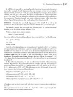
Let us consider some examples to illustrate these concepts.
The
examples are based
on a
much
simplified variation of
the
COMPANY

database application from Figure 5.7,
which
2.
An
example would be a temporal
event
specified as a periodic time, such as: Trigger this rule
every day at 5:30
A.M.
758
I
Chapter
24
Enhanced
Data
Models
for
Advanced
Applications
is
shown
in Figure 24.1,
with
each
employee
having
a
name
(NAME),
social security number

(SSN),
salary
(SALARY),
department
to
which
they
are currently assigned
(DNO,
a foreign key
to
DEPARTMENT),
and
a direct supervisor
(SUPERVISOR_SSN,
a (recursive) foreign key to
EMPLOYEE).
For this example, we assume
that
null is allowed for
DNO,
indicating
that
an
employee may be temporarily unassigned to any
department.
Each
department
has a
name

(DNAME),
number
(DNO),
the
total
salary of all employees assigned to
the
department
(TOTAL_SAL),
and
a manager
(MANAGER_SSN,
a foreign key to
EMPLOYEE).
Notice
that
the
TOTAL_SAL
attribute
is really a derived attribute, whose value should be
the
sum of
the
salaries of all employees who are assigned to
the
particular department.
Maintaining
the
correct
value of such a derived

attribute
can
be
done
via
an
active rule.
We first
have
to
determine
the
events
that
may cause a
change
in
the
value of
TOTAL_SAL,
which
are as follows:
1. Inserting
(one
or more)
new
employee tuples.
2.
Changing
the

salary of
(one
or more) existing employees.
3.
Changing
the
assignment of existing employees from
one
department
to another.
4.
Deleting
(one
or more) employee tuples.
In
the
case of
event
1, we only
need
to
recompute
TOTAL_SAL
if
the
new
employee is
immediately assigned to a
department-that
is, if

the
value of
the
DNO
attribute
for the
new
employee tuple is
not
null
(assuming
null
is allowed for
DNO).
Hence,
this would be
the
condition to be checked. A similar
condition
could be
checked
for
event
2 (and 4) to
determine
whether
the
employee whose salary is
changed
(or who is being deleted) is

currently assigned to a
department.
For
event
3, we will always execute
an
action to
maintain
the
value of
TOTAL_SAL
correctly, so no
condition
is
needed
(the
action
is
always
executed).
The
action for
events
1, 2,
and
4 is to automatically update
the
value
ofTOTAL_SAL
for

the
employee's
department
to reflect
the
newly inserted, updated, or deleted employee's
salary. In
the
case of
event
3, a twofold
action
is needed;
one
to
update
the
TOTAL_SAL
of
the
employee's old
department
and
the
other
to update
the
TOTAL_SAL
of
the

employee's
new
department.
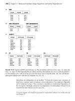
The
four active rules (or triggers) R1, R2, R3,
and
R4-corresponding
to
the
above
situation-can
be specified in
the
notation
of
the
Oracle
DBMSas
shown
in Figure 24.2a.
Let us consider rule R1 to illustrate
the
syntax of creating triggers in Oracle.
The
CREATE
EMPLOYEE
I NAME
~~~ERVISOR_SS~
DEPARTMENT
IDNAME

~
TOTAL_SAL]
MAN~~E~=-SSN
J
FIGURE 24.1 A
simplified
COMPANY
database
used
for
active
rule
examples.
24.1
Active
Database Concepts and Triggers I
759
(a) RI: CREATE TRIGGER TOTALSAL1
AFTER INSERT ON EMPLOYEE
FOR EACH ROW
WHEN (NEW.DNO IS NOT NULL)
UPDATE
DEPARTMENT
SET TOTAL_SAL=TOTAL_SAL + NEW.SALARY
WHERE
DNO=NEW.DNO;
R2: CREATE TRIGGER TOTALSAL2
AFTER UPDATE OF SALARY ON EMPLOYEE
FOR EACH ROW
WHEN (NEW.DNO IS NOT NULL)

UPDATE
DEPARTMENT
SET TOTAL_SAL=TOTAL_SAL + NEW.SALARY - OLD.SALARY
WHERE DNO=NEW.DNO;
R3: CREATE TRIGGER TOTALSAL3
AFTER UPDATE OF DNO ON EMPLOYEE
FOR EACH ROW
BEGIN
UPDATE
DEPARTMENT
SET TOTAL_SAL=TOTAL_SAL + NEW.SALARY
WHERE DNO=NEW.DNO;
UPDATE DEPARTMENT
SET TOTAL_SAL=
TOTAL_SAL-
OLD.SALARY
WHERE DNO=OLD.DNO;
END;
R4: CREATE TRIGGER
TOTALSAL4
AFTER DELETE ON EMPLOYEE
FOR EACH ROW
WHEN (OLD.DNO IS NOT NULL)
UPDATE
DEPARTMENT
SET TOTAL_SAL=TOTAL_SAL - OLD.SALARY
WHERE DNO=OLD.DNO;
(b)
RS: CREATE TRIGGER INFORM_SUPERVISOR1
BEFORE INSERT OR UPDATE OF SALARY, SUPERVISOR_SSN ON EMPLOYEE

FOR EACH
ROW
WHEN
(NEW.SALARY > (SELECT SALARY FROM EMPLOYEE
WHERE SSN=NEW.SUPERVISOR_SSN))
INFORM_SUPERVISOR(NEW. SUPERVISOR_SSN, NEW.SSN);
FIGURE
24.2
Specifying active rules as triggers in
Oracle
notation. (a) Triggers for
automatically
maintaining
the consistency
of
TOTAL_SAL
of DEPARTMENT. (b) Trigger for
comparing an employee's salary
with
that of his or her supervisor.
760 I
Chapter
24 Enhanced
Data
Models
for
Advanced
Applications
TRIGGER
statement

specifies a trigger (or active rule)
name-TOTALSALl
for
Rl.
The
AFTER-clause specifies
that
the
rule will be triggered after
the
events
that
trigger the rule
occur.
The
triggering
events-an
insert of a
new
employee in this
example-are
specified
following
the
AFTER
keyword."
The
ON-clause specifies
the
relation

on
which
the
rule is
specified-EMPLOYEE
for
Rl.
The
optional
keywords
FOR
EACH
ROW
specify
that
the
rule will
be triggered
oncefor eachrow
that
is affected by
the
triggering
event."
The
optional
WHEN-
clause is used to specify any
conditions
that

need
to
be
checked
after
the
rule is triggered
but
before
the
action
is executed. Finally,
the
actionts)
to
be
taken
are specified as a
PL!
SQL
block,
which
typically
contains
one
or more
SQL
statements
or calls to execute
external

procedures.
The
four triggers (active rules)
Rl
, R2, R3,
and
R4 illustrate a
number
of features of
active rules. First,
the
basic
events
that
can
be specified for triggering
the
rules are the
standard
SQL
update commands:
INSERT,
DELETE,
and
UPDATE.
These
are specified by the
keywords INSERT,
DELETE,
and

UPDATE in
Oracle
notation.
In
the
case of
UPDATE
one
may specify
the
attributes
to
be
updated-for
example, by writing UPDATEOF
SALARY,
DND.
Second,
the
rule designer needs
to
have
a way to refer to
the
tuples
that
have been
inserted, deleted, or modified by
the
triggering

event.
The
keywords NEW
and
OLD
are
used in
Oracle
notation;
NEW
is used to refer to a newly inserted or newly updated tuple,
whereas
OLD
is used to refer to a
deleted
tuple or to a tuple before it was updated.
Thus
rule
Rl
is triggered after
an
INSERT
operation
is applied to
the
EMPLOYEE
relation.
In
Rl,
the

condition
(NEW.
DNO
IS
NOT
NULL)
is checked,
and
if it evaluates to true, meaning
that
the
newly inserted employee tuple is related to a
department,
then
the
action is
executed.
The
action
updates
the
DEPARTMENT
tuplets) related
to
the
newly inserted
employee by adding
their
salary
(NEW.

SALARY)
to
the
TOTAL_SAL
attribute
of
their
related
department.
Rule R2 is similar to
Rl,
but
it is triggered by an
UPDATE
operation
that
updates the
SALARY
of
an
employee
rather
than
by
an
INSERT.
Rule R3 is triggered by
an
update to the
DNO

attribute
of
EMPLOYEE,
which
signifies
changing
an
employee's assignment from one
department
to another.
There
is
no
condition
to
check
in R3, so
the
action
is executed
whenever
the
triggering
event
occurs.
The
action
updates
both
the

old department and
new
department
of
the
reassigned employees by adding
their
salary to
TOTAL_SAL
of their
new
department
and
subtracting
their
salary from
TOTAL_SAL
of
their
olddepartment. Note
that
this should work
even
if
the
value of
DNO
was null, because in this case no department
will be selected for
the

rule
action.i
It is
important
to
note
the
effect of
the
optional
FOR
EACH
ROW
clause, which
signifies
that
the
rule is triggered separately for each tuple.
This
is
known
as a row-level
trigger.
If
this clause was left out,
the
trigger would be
known
as a
statement-level

trigger


~

~-



3. As we shall see later, it is also possible
to
specify
BEFORE
instead of AITER, which indicates that
the rule istriggered
before
the
triggering
event is executed.
4. Again, we shall see later that an alternative is
to
trigger the rule only once even ifmultiple
rows
(tuples) are affectedby the triggeringevent.
5. Rl, R2, and R4 can also be written without a condition. However, they may be more
efficient
to
execute with the condition since the action is not invoked unlessit isrequired.
24.1
Active

Database Concepts and Triggers I 761
and would be triggered
once
for
each
triggering
statement.
To see
the
difference, consider
the
following update operation,
which
gives a 10
percent
raise to all employees assigned
to
department
5.
This
operation
would be an
event
that
triggers rule R2:
UPDATE
SET
WHERE
EMPLOYEE
SALARY =

1.
1 *
SALARY
DNO
=
5;
Because
the
above
statement
could update multiple records, a rule using row-level
semantics, such as R2 in Figure 24.2, would be triggered
once for eachrow, whereas a rule
using statement-level semantics is triggered
only once.
The
Oracle system allows
the
user to
choose
which
of
the
above two options is to be used for
each
rule. Including
the
optional
FOR EACH ROW clause creates a row-level trigger,
and

leaving it
out
creates a statement-
level trigger.
Note
that
the
keywords NEW
and
OLD
can
only be used with row-level triggers.
As a second example, suppose we want to check whenever an employee's salary is greater
than
the
salary of his or
her
direct supervisor. Several events
can
trigger this rule: inserting a
new employee, changing an employee's salary,or changing an employee's supervisor. Suppose
that the action to take would be
to call an external procedure
INFORM_SUPERVISOR,6
which will
notify the supervisor.
The
rule could
then
be written as in R5 (see Figure 24.2b).

Figure 24.3 shows the syntax for specifying some of the main options available in Oracle
triggers.We will describe the syntax for triggers in the
sQL-99
standard in Section 24.1.5.
24.1.2 Design and Implementation Issues for
Active Databases
The
previous
section
gave an overview of some of
the
main
concepts for specifying active
rules. In
this
section, we discuss some additional issues
concerning
how rules are designed
and implemented.
The
first issue concerns activation, deactivation,
and
grouping of rules.
<trigger> ::= CREATETRIGGER<trigger name>
(AFTERI BEFORE) <triggering events> ON <table name>
[ FOR EACHROW1
[ WHEN <condition> 1
<trigger actions> ;
<triggering events> ::=<trigger event> {OR <trigger event> }
<trigger event>::=INSERT

I DELETEI UPDATE
[OF
<column name> {, <column names} 1
<trigger action>
::=<PUSQL
block>
FIGURE
24.3
A syntax summary for specifying triggers in the
Oracle
system (main
options only).
6. Assuming
that
an appropriate
external
procedure has
been
declared.
This
is a feature
that
is now
available in
SQL.
762
I Chapter 24 Enhanced Data Models for Advanced Applications
In
addition
to creating rules, an active database system should allow users

to
activate,
deactivate,
and
drop
rules by referring to
their
rule names. A deactivated
rule
will not be
triggered by
the
triggering event.
This
feature allows users
to
selectively deactivate rules
for
certain
periods of time
when
they are
not
needed.
The
activate
command
will make
the
rule active again.

The
drop
command
deletes
the
rule from
the
system. Another
option
is to group rules
into
named
rule
sets, so
the
whole set of rules could be activated,
deactivated, or dropped.
It
is also useful to
have
a
command
that
can
trigger a rule or rule
set via an explicit
PROCESS RULES
command
issued by
the

user.
The
second issue concerns whether
the
triggered action should be executed
before,
after,
or
concurrently
withthe triggering event. A related issue is whether the action being executed
should be considered as a
separate
transaction
or whether it should be part of the
same
transaction
that
triggered the rule. We will first try to categorize the various options. It is
important to note
that
not
all options may be available for a particular active database
system.
In fact, most commercial systems are
limited
to oneor twoof
the
options
that
we will now

discuss.
Let us assume
that
the
triggering
event
occurs as
part
of a transaction execution. We
should first consider
the
various options for how
the
triggering
event
is related to the
evaluation
of
the
rule's condition.
The
rule condition evaluation is also
known
as rule
consideration,
since
the
action
is to be
executed

only after considering whether the
condition
evaluates to true or false.
There
are
three
main
possibilities for rule
consideration:
1.
Immediate
consideration:
The
condition
is evaluated as
part
of
the
same transaction
as
the
triggering
event,
and
is evaluated immediately.
This
case
can
be further cat-
egorized

into
three
options:
• Evaluate
the
condition
before
executing
the
triggering event.
• Evaluate
the
condition
after executing
the
triggering event.
• Evaluate
the
condition
instead
of executing
the
triggering event.
2. Deferred
consideration:
The
condition
is evaluated at
the
end

of
the
transaction
that
included
the
triggering event. In this case,
there
could be many triggered
rules waiting to
have
their
conditions evaluated.
3. Detached
consideration:
The
condition
is evaluated as a separate transaction,
spawned from
the
triggering transaction.
The
next
set of options concerns
the
relationship between evaluating the
rule
condition
and
executing

the
rule action. Here, again, three options are possible: immediate,
deferred, and detached execution. However, most active systems use
the
first option. That
is, as soon as
the
condition is evaluated, if it returns true, the action is
immediately
executed.
The
Oracle system (see
Section
24.1.1) uses
the
immediate
consideration
model, but it
allows
the
user
to
specify for
each
rule
whether
the
before
or after
option

is to be used with
immediate
condition
evaluation.
It
also uses
the
immediate
execution model. The
STARBURST system (see
Section
24.1.3) uses
the
deferred
consideration
option, meaning
that
all rules triggered by a transaction wait
until
the
triggering transaction reaches its
end
and
issues its COMMIT WORK
command
before
the
rule conditions are
evaluated.I

-



7.STARBURST also
allows
the user
to
explicitly startruleconsideration viaa PROCESS
RULES
command.
24.1
Active
Database Concepts and Triggers I 763
Another
issue
concerning
active database rules is
the
distinction between row-level
rules
versus statement-level
rules.
Because
SQL
update statements
(which
act

as triggering
events)
can
specify a set of tuples,
one
has to distinguish between
whether
the
rule should
be considered
once
for
the
wholestatement or
whether
it should be considered separately
for eachrow
(that
is, tuple) affected by
the
statement.
The
sQL-99 standard (see
Section
24.1.5)
and
the
Oracle
system (see
Section

24.1.1) allow
the
user to choose
which
of
the
above two options is to be used for
each
rule, whereas STARBURST uses statement-level
semantics only. We will give examples of
how
statement-level triggers
can
be specified in
Section 24.1.3.
One
of
the
difficulties
that
may
have
limited
the
widespread use of active rules, in
spite of
their
potential
to simplify database
and

software development, is
that
there are no
easy-to-use techniques for designing, writing,
and
verifying rules. For example, it is quite
difficult
to
verify
that
a set of rules is
consistent,
meaning
that
two or more rules in
the
set
do
not
contradict
one
another.
It
is also difficult to guarantee
termination
of a set of rules
under all circumstances. To briefly illustrate
the
termination
problem, consider

the
rules
in Figure 24.4. Here, rule
Rl
is triggered by an INSERT
event
on TABLEl
and
its
action
includes an
update
event
on
ATTRIBUTEl of TABLE2. However, rule R2's triggering
event
is an
UPDATE
event
on
ATTRIBUTEl of TABLE2,
and
its
action
includes an INSERT
event
on TABLEl.
It is easy
to
see in this example

that
these two rules
can
trigger
one
another
indefinitely,
leading to
nontermination.
However, if dozens of rules are written, it is very difficult to
determine
whether
termination
is guaranteed or
not.
If active rules are to reach
their
potential, it is necessary to develop tools for
the
design, debugging,
and
monitoring
of active rules
that
can
help
users in designing and
debugging
their
rules.

24.1.3
Examples of
Statement-level
Active
Rules
in
STARBURST
We
now
give some examples
to
illustrate
how
rules
can
be specified in
the
STARBURST
experimental DBMS.
This
will allow us
to
demonstrate how statement-level rules
can
be
written, since these are
the
only types of rules allowed in STARBURST.
RI: CREATE TRIGGER T1
AFTER INSERT ON TABLE1

FOR EACH ROW
UPDATE TABLE2
SET ATIRIBUTE1= ;
R2: CREATE TRIGGER T2
AFTER UPDATE OF ATIRIBUTE1 ON TABLE2
FOR EACH ROW
INSERT INTO TABLE1 VALUES ( );
FIGURE
24.4
An example to illustrate the
termination
problem
for active rules.
764
I Chapter 24 Enhanced Data
Models
for
Advanced
Applications
The
three
active rules
RlS,
R2S,
and
R3S in Figure 24.5
correspond
to
the
first three

rules in Figure
24.2,
but
use
STARBURST
notation
and
statement-level
semantics. We can
explain
the
rule
structure
using rule
RlS.
The
CREATE
RULE
statement
specifies a rule
name-TOTALSALl for
RlS.
The
ON-clause specifies
the
relation
on
which
the
rule is

specified-EMPLOYEE
for
RlS.
The
WHEN-clause is used to specify
the
events
that
trigger
the
rule.f
The
optional
IF-clause is used
to
specify any
conditions
that
need
to be checked,
RIS: CREATE RULE TOTALSAL1 ON EMPLOYEE
WHEN INSERTED
IF EXISTS(SELECT· FROM INSERTED WHERE
DNO IS NOT NULL)
THEN UPDATE
DEPARTMENT AS D
SET D.TOTAL_SAL=D.TOTAL_SAL +
(SELECT SUM(I.SALARY) FROM INSERTED AS I WHERE D.DNO =
I.ONO)
WHERE D.DNO IN (SELECT DNO FROM INSERTED);

R2S: CREATE RULE
TOTALSAL2 ON EMPLOYEE
WHEN
IF
THEN
UPDATED (SALARY)
EXISTS(SELECT· FROM NEW·UPDATED WHERE DNO IS NOT NULL)
OR EXISTS(SELECT· FROM OLD·UPDATED WHERE DNO IS NOT NULL)
UPDATE
DEPARTMENT AS D
SET D.TOTAL_SAL=D.TOTAL_SAL +
(SELECT SUM(N.SALARY) FROM NEW-UPDATED AS N WHERE
D.DNO =N,DNO) -
(SELECT SUM(O,SALARY) FROM OLD-UPDATED AS 0 WHERE
D.DNO=O.DNO)
WHERE D.DNO IN (SELECT DNO FROM NEW-UPDATED) OR
D,DNO IN (SELECT DNO FROM OLD-UPDATED);
R3S: CREATE RULE
TOTALSAL3 ON EMPLOYEE
WHEN UPDATED(DNO)
THEN UPDATE
DEPARTMENT AS D
SET D.TOTAL_SAL=D.TOTAL_SAL +
(SELECT SUM(N.SALARY) FROM NEW-UPDATED AS N WHERE
D.DNO=N.DNO)
WHERE D.DNO IN (SELECT DNO FROM NEW-UPDATED);
UPDATE
DEPARTMENT AS D
SET D.TOTAL_SAL=D.TOTAL_SAL-
(SELECT SUM(O.SALARY) FROM OLD-UPDATED AS 0 WHERE

O.DNO=O.DNO)
WHERE D.DNO IN (SELECT DNO FROM OLD-UPDATED);
FIGURE
24.5
Active
rules using statement-level semantics in
STARBURST
notation.
8. Note that the
WHEN
keywordspecifies events in
STARBURST
but is used to
specify
the rule
condi-
tionin SQLand Oracle triggers.
24.1 Active Database Concepts and Triggers I
765
Finally,
the
THEN-clause is used to specify
the
action
(or actions)
to
be taken, which are
typically
one
or more

SQL
statements.
In
STAR
BURST,
the
basic
events
that
can
be specified for triggering
the
rules are
the
standard
SQL
update commands:
INSERT,
DELETE,
and
UPDATE.
These
are specified by
the
keywords INSERTED, DELETED,
and
UPDATED in ST
ARBURST
notation.
Second,

the
rule designer
needs to
have
a way to refer to
the
tuples
that
have
been
modified.
The
keywords INSERTED,
DELETED, NEW-UPDATED,
and
OLD-UPDATED are used in ST
ARBURST
notation
to refer to four
transition
tables (relations)
that
include
the
newly inserted tuples,
the
deleted tuples,
the
updated tuples
before

they were updated,
and
the
updated tuples after
they
were updated,
respectively. Obviously, depending on
the
triggering events, only some of these transition
tables may be available.
The
rule writer
can
refer to these tables
when
writing
the
condition
and
action
parts of
the
rule. Transition tables
contain
tuples of
the
same type as
those in
the
relation

specified in
the
ON-clause of
the
rule-for
RlS,
R2S,
and
R3S, this
is
the
EMPLOYEE
relation.
In statement-level semantics,
the
rule designer
can
only refer
to
the
transition tables
as a whole
and
the
rule is triggered only once, so
the
rules must be
written
differently
than

for row-level semantics. Because multiple employee tuples may be inserted in a single
insert
statement,
we
have
to
check
if at
least
one of
the
newly inserted employee tuples is
related to a
department.
In
RlS,
the
condition
EXISTSCSELECT
*
FROM
INSERTED
WHERE
DNO
IS
NOT
NULL)
ischecked,
and
if it evaluates to true,

then
the
action
is executed.
The
action
updates in a
single
statement
the
DEPARTMENT
tupleis) related to
the
newly inserted emploveets) by add-
ing
their
salaries to
the
TOTAL_SAL
attribute
of
each
related department. Because more
than
one newly inserted employee may belong to
the
same
department,
we use
the

SUM
aggre-
gate
function
to ensure
that
all
their
salaries are added.
Rule
R2S
is similar to
RlS,
but
is triggered by an
UPDATE
operation
that
updates
the
salary of
one
or more employees
rather
than
by an
INSERT.
Rule R3S is triggered by an
update to
the

DNO
attribute
of
EMPLOYEE,
which
signifies changing
one
or more employees'
assignment from
one
department
to another.
There
is no
condition
in R3S, so
the
action
is executed
whenever
the
triggering
event
occurs.l'
The
action
updates
both
the
old

departmentfs)
and
new
departmentts)
of
the
reassigned employees by adding
their
salary
to
TOTAL_SAL of
each
new
department
and
subtracting
their
salary from TOTAL_SAL of
each
old
department.
In our example, it is more complex to write
the
statement-level rules
than
the
row-
level rules, as
can
be illustrated by comparing Figures 24.2

and
24.5. However, this is
not
a general rule,
and
other
types of active rules may be easier to specify using statement-
level
notation
than
when
using row-level
notation.
The
execution model for active rules in
STARBURST
usesdeferred consideration.
That
is,
all the rules
that
are triggered within a transaction are placed in a set ealled the conflict
9. As in
the
Oracle
examples, rules R1S
and
R2S
can
be

written
without
a condition. However,
they may be more efficient
to
execute
with
the
condition
since
the
action
is
not
invoked unless it is
required.
766 IChapter 24 Enhanced Data Models for Advanced Applications
set-which
is
not
considered for evaluation of conditions and execution until the transaction
ends (by issuing its
COMMIT WORKcommand).
STARBURST
also allows the user to explicitly
start rule consideration in the middle of a transaction via an explicit
PROCESS
RULES
command. Because multiple rules must be evaluated, it isnecessary
to

specify an order among
the
rules.
The
syntax for rule declaration in ST
ARBURST
allows
the
specification of
ordering
among the rules to instruct
the
system about the order in which a set of rules should be
considered.l" In addition, the transition
tables-INSERTED,
DELETED,
NEW-UPDATED,
and
OLD-
UPDATED eontain
the net
effect
of all the operations within the transaction
that
affected each
table, since multiple operations may have been applied to each table during the transaction.
24.1.4 Potential Applications for Active Databases
We now briefly discuss some of
the
potential

applications of active rules. Obviously, one
important
application is to allow notification of
certain
conditions
that
occur. For
exam-
ple, an active database may be used to monitor, say,
the
temperature of an industrial
fur-
nace.
The
application
can
periodically insert in
the
database
the
temperature
reading
records directly from temperature sensors,
and
active rules
can
be written
that
are
trig-

gered
whenever
a temperature record is inserted,
with
a
condition
that
checks if the
tem-
perature exceeds
the
danger level,
and
the
action
to raise an alarm.
Active
rules
can
also be used to enforce integrity constraints by specifying the
types
of
events
that
may cause rhe constraints to be violated and
then
evaluating appropriate
conditions
that
check whether

the
constraints are actually violated by the event or not.
Hence, complex application constraints, often
known
as business rules may be
enforced
that
way. For example, in
the
UNIVERSITY
database application, one rule may monitor the
grade
point
average of students whenever a new grade is entered, and it may alert the
advisor if
the
CPA
of a student falls below a certain threshold;
another
rule may check that
course prerequisites are satisfied before allowing a student to enroll in a course; and so on.
Other
applications include
the
automatic maintenance of derived data, such as the
examples of rules
R1 through R4
that
maintain
the

derived attribute
TOTAL_SAL
whenever
individual employee tuples are changed. A similar application is
to
use active
rules
to
maintain
the
consistency of materialized views (see
Chapter
9) whenever the base
relations
are modified.
This
application is also relevant to the new data warehousing technologies
(see
Chapter
28). A related application is to maintain replicated tables consistent
by
specifying rules
that
modify
the
replicas whenever
the
master table is modified.
24.1.5 Triggers in SQL-99
Triggers in

the
sQL-99
standard are quite similar to
the
examples we discussed in Section
24.1.1,
with
some
minor
syntactic differences.
The
basic
events
that
can
be specified
for
triggering
the
rules are
the
standard SQL update commands: INSERT,
DELETE,
and
UPDATE.
-~~ ~~~~~~ ~ ~~ _._ ~~
10.
If
no order is specified between a pair of rules,
the

system default order is based on placing the
rule declared first ahead of
the
other
rule.
24.2 Temporal Database Concepts I
767
In
the
case of
UPDATE
one
may specify
the
attributes to be updated.
Both
row-level
and
statement-level triggers are allowed, indicated in
the
trigger by
the
clauses
FOR
EACH
ROWand
FOR
EACH
5T
ATEMENT,

respectively.
One
syntactic difference is
that
the
trigger
may specify particular tuple variable names for
the
old
and
new
tuples instead of using
the
keywords
NEW
and
OLD
as in Figure 24.1. Trigger
Tl
in Figure 24.6 shows
how
the
row-
level trigger R2 from Figure 24.1(a) may be specified in 5QL-99. Inside
the
REFERENCING
clause, we
named
tuple variables (aliases) 0
and

N to refer to
the
OLD
tuple (before mod-
ification)
and
NEW
tuple (after modification), respectively. Trigger T2 in Figure 24.6
shows
how
the
statement-level
trigger R2S from Figure 24.5 may be specified in 5QL-99.
For a
statement-level
trigger,
the
REFERENCING
clause is used to refer to
the
table of all
new tuples (newly inserted or newly updated) as
N, whereas
the
table of all old tuples
(deleted tuples or tuples before they were updated) is referred to as O.
24.2
TEMPORAL
DATABASE CONCEPTS
Temporal databases, in

the
broadest sense, encompass all database applications
that
require some aspect of
time
when
organizing
their
information.
Hence,
they provide a
good example to illustrate
the
need
for developing a set of unifying concepts for applica-
tion
developers to use. Temporal database applications
have
been
developed since
the
early days of database usage. However, in creating these applications, it was mainly left
to
T1:
CREATE
TRIGGER
TOTALSAL1
AFTER
UPDATE
OF

SALARY
ON
EMPLOYEE
REFERENCING
OLD
ROW
AS
0,
NEW
ROW
AS
N
FOR
EACH
ROW
WHEN
(N.DNO
IS
NOT
NULL)
UPDATE
DEPARTMENT
SET
TOTAL_SAL
=
TOTAL
SAL
+
N.SALARY
-

O.SALARY
WHERE
DNO
=
N.DNO;
T2:
CREATE
TRIGGER
TOTALSAL2
AFTER
UPDATE
OF
SALARY
ON
EMPLOYEE
REFERENCING
OLD
TABLE
AS
0,
NEW
TABLE
AS
N
FOR
EACH
STATEMENT
WHEN
EXISTS(SELECT
*

FROM
N
WHERE
N.DNO
IS
NOT
NULL)
OR
EXISTS(SELECT
*
FROM
0
WHERE
O.DNO
IS
NOT
NULL)
UPDATE
DEPARTMENT
AS
D
SET
D.TOTAL_SAL
=
D.TOTAL_SAL
+
(SELECT
SUM(N.SALARY)
FROM
N

WHERE
D.DNO=N.DNO)
-
(SELECT
SUM(O.SALARY)
FROM
0
WHERE
D.DNO=O.DNO)
WHERE
DNO
IN
((SELECT
DNO
FROM
N)
UNION
(SELECT
DNO
FROM
0));
FIGURE
24.6
Trigger T1 illustrating the syntax for defining triggers in sQL-99.
768 I
Chapter
24
Enhanced
Data
Models

for
Advanced
Applications
the
application designers
and
developers to discover, design, program,
and
implement the
temporal concepts they need.
There
are many examples of applications where some
aspect of time is
needed
to
maintain
the
information in a database.
These
include
health-
care, where
patient
histories
need
to be maintained; insurance, where claims
and
accident
histories are required as well as information
on

the
times
when
insurance policies are in
effect;
reservation systemsin general (hotel, airline, car rental, train, etc.}, where informa-
tion
on
the
dates
and
times
when
reservations are in effect are required;
scientific
data-
bases,
where
data
collected from experiments includes
the
time
when
each
data is
measured; an so on. Even
the
two examples used in this book may be easily expanded into
temporal applications. In
the

COMPANY
database, we may wish to keep
SALARY,
JOB, and
PROJECT
histories
on
each
employee. In
the
UNIVERSITY database, time is already included in the
SEMESTER
and
YEAR
of
each
SECTION
of a
COURSE;
the
grade history of a
STUDENT;
and
the
informa-
tion
on
research grants. In fact, it is realistic
to
conclude

that
the
majority of database
applications
have
some temporal information. Users
often
attempted
to simplify or ignore
temporal aspects because of
the
complexity
that
they
add to
their
applications.
In this section, we will introduce some of
the
concepts
that
have
been
developed to
deal
with
the
complexity of temporal database applications.
Section
24.2.1 gives an

overview of how time is represented in databases,
the
different types of temporal
information,
and
some of
the
different dimensions of time
that
may be needed. Section
24.2.2 discusses
how
time
can
be incorporated
into
relational databases.
Section
24.2.3
gives some additional options for representing time
that
are possible in database
models
that
allow complex-structured objects, such as object databases.
Section
24.2.4 introduces
operations for querying temporal databases,
and
gives a brief overview of the

TSQL2
language,
which
extends SQL with temporal concepts.
Section
24.2.5 focuses on time
series data,
which
is a type of temporal
data
that
is very
important
in practice.
24.2.1 Time Representation, Calendars, and
Time
Dimensions
For temporal databases, time is considered to be an
ordered
sequence
of points in
some
granularity
that
is
determined
by
the
application. For example, suppose
that

some
tempo-
ral application
never
requires time units
that
are less
than
one
second.
Then,
each time
point
represents
one
second in time using this granularity. In reality,
each
second is a
(short)
timeduration,
not
a point, since it may be further divided
into
milliseconds,
micro-
seconds,
and
so on. Temporal database researchers
have
used

the
term
chronon
instead of
point
to describe this
minimal
granularity for a particular application.
The
main
conse-
quence
of choosing a
minimum
granularity-say,
one
second-is
that
events occurring
within
the
same second will be considered to be simultaneous events,
even
though in
real-
ity they may
not
be.
Because there is no known beginning or ending of time, one needs a reference point
from

which
to measure specific time points. Various calendars are used by various
cultures
(such as Gregorian (Western), Chinese, Islamic, Hindu, Jewish, Coptic, etc.) with
different
reference points. A calendar organizes time into different time units for convenience.
Most
24.2 Temporal Database Concepts I 769
calendars group 60 seconds into a minute, 60 minutes into an hour, 24 hours into a day
(based on the physical time of earth's rotation around its axis),
and
7 days into a week.
Further grouping of days into
months
and
months
into years either follow solar or lunar
natural
phenomena,
and
are generally irregular. In
the
Gregorian calendar,
which
is used in
most Western countries, days are grouped into
months
that
are either
28,29,30,

or 31 days,
and 12
months
are grouped
into
a year. Complex formulas are used to map
the
different
time units to
one
another.
In
sQL2,
the
temporal
data
types (see
Chapter
8) include DATE (specifying Year,
Month,
and
Day as YYYY-MM-DD),
TIME
(specifying Hour,
Minute,
and
Second
as
HH:MM:SS), TIMESTAMP (specifying a Date/Time combination,
with

options for including
sub-second divisions if they are needed),
INTERVAL (a relative time duration, such as 10
days or
250
minutes),
and
PERIOD
(an
anchored
time
duration
with
a fixed starting point,
such as
the
lO-day period from January 1, 1999, to January 10, 1999, inclusive).ll
Event Information Versus Duration (or State) Information. A
temporal
database
will store
information
concerning
when
certain
events
occur, or
when
certain
facts are

considered to be true.
There
are several
different
types of
temporal
information.
Point
events
or
facts
are typically associated in
the
database
with
a single
time
point
in
some granularity. For
example,
a
bank
deposit
event
may be associated
with
the
timestamp
when

the
deposit
was made, or
the
total
monthly
sales
of
a
product
(fact}
may be associated
with
a
particular
month
(say, February 1999).
Note
that
even
though
such
events
or facts may
have
different granularities,
each
is still associated
with
a

single
time value in
the
database.
This
type of
information
is
often
represented
as
time
series
data
as we
shall
discuss in
Section
24.2.5.
Duration
events
or
facts,
on
the
other
hand,
are associated
with
a specific

time
period
in
the
database.l/
For example,
an employee may
have
worked in a
company
from
August
15, 1993, till
November
20, 1998.
A
time
period
is represented by its
start
and
end
time
points
[START-TIME,
END-TIME].
For example,
the
above period is represented as
[1993-08-15,

1998-11-20].
Such
a time
period is
often
interpreted
to
mean
the
set of all time
points
from start-time to end-time,
inclusive, in
the
specified granularity.
Hence,
assuming day granularity,
the
period
[1993-
08-15,
1998-11-20]
represents
the
set of all days from August 15, 1993,
until
November
20, 1998, inclusive.13
11. Unfortunately,
the

terminology has
not
been
used consistently. For example,
the
term
intervalis
often used to
denote
an
anchored
duration. For consistency, we shall use
the
SQL terminology.
12.
This
is
the
same as an
anchored
duration.
It
has also
been
frequently called a
time
interval,
but
to avoid confusion we will use
period

to be
consistent
with
SQL terminology.
13.
The
representation
[1993-08-15,
1998-11-20]
is called a
closed
interval representation.
One
can also use an open interval,
denoted
[1993-08-15,
1998-11-21),
where
the
set of points
does
not
include
the
end
point.
Although
the
latter
representation

is sometimes more
convenient,
we shall
use closed intervals
throughout
to avoid confusion.
770 I
Chapter
24 Enhanced Data Models for
Advanced
Applications
Valid Time and Transaction Time
Dimensions.
Given
a particular event or
fact
that
is associated
with
a particular time
point
or time period in
the
database, the
association may be interpreted to
mean
different things.
The
most
natural

interpretation
is
that
the
associated time is
the
time
that
the
event
occurred, or
the
period during which
the
fact was considered to be true in the real world.
If
this
interpretation
is used, the
associated
time
is often referred to as
the
valid time. A temporal database using this
interpretation
is called a valid time database.
However, a different
interpretation
can
be used, where

the
associated time refers to
the
time
when
the
information was actually stored in
the
database;
that
is, it is the value
of
the
system time clock
when
the
information is valid in the system. 14 In this case, the
associated time is called
the
transaction
time. A temporal database using this
interpretation
is called a
transaction
time database.
Other
interpretations
can
also be intended,
but

these two are considered to be the
most
common
ones,
and
they are referred to as time dimensions. In some applications,
only
one
of
the
dimensions is
needed
and
in
other
cases
both
time dimensions are
required, in which case
the
temporal database is called a
bitemporal
database. If other
interpretations are
intended
for time,
the
user
can
define

the
semantics
and
program the
applications appropriately,
and
it is called a user-defined time.
The
next
section shows
with
examples
how
these concepts
can
be incorporated into
relational databases,
and
Section
24.2.3 shows an approach to incorporate temporal
concepts
into
object
databases.
24.2.2 Incorporating Time in Relational Databases
Using Tuple Versioning
Valid Time Relations. Let us now see how
the
different types of temporal databases
may be represented in

the
relational model. First, suppose
that
we would like to include
the
history of changes as they occur in
the
real world. Consider again
the
database in
Figure 24.1,
and
let us assume
that,
for this application,
the
granularity is day. Then,
we
could
convert
the
two relations
EMPLOYEE
and
DEPARTMENT
into
valid
time
relations by
adding

the
attributes VST (Valid
Start
Time)
and
VET (Valid End Time), whose
data
type is
DATE
in order to provide day granularity.
This
is shown in Figure 24.7a, where
the
relations
have
been
renamed
EMP
_VT
and
DEPT_VT, respectively.
Consider
how
the
EMP
_VT
relation differs from
the
nontemporal
EMPLOYEE

relation
(Figure 24.1)
.15 In
EMP
_VT,
each
tuple V represents a
version
of an employee's information
that
is valid
(in
the
real world) only during
the
time period
[v.
VST,
V.
VET],
whereas in
EMPLOYEE
each
tuple represents only
the
current
state or
current
version of
each

employee.
In
EMP
_VT,
the
current
version
of
each
employee typically has a special value, now, as its
14.The explanation is more involved, as weshallsee in Section 24.2.3.
15. A nontemporal relation isalsocalled a snapshot relation asit
shows
only the current
snapshot
or
currentstateof the database.
24.2
Temporal Database Concepts I 771
(a)
EMP_VT
SUPERVISOR_SSN
DEPT_VT
I DNAME
~
TOTAL_SAL IMANAGER_SSN
~
SUPERVISOR_SSN
DEPT_TT
I DNAME

~
TOTAL_SAL I MANAGER_SSN
~
(c)
EMP_BT
SUPERVISOR_SSN
DEPT_BT
FIGURE
24.7
Different types of temporal relational databases. (a) Valid time data-
base
schema.
(b) Transaction time
database
schema.
(c) Bitemporal
database
schema.
valid
end
time.
This
special value, now, is a temporal variable
that
implicitly represents
the
current
time as time progresses.
The
nontemporal

EMPLOYEE
relation would only
include those tuples from
the
EMP
_VT
relation whose VET is now.
Figure 24.8 shows a few tuple versions in
the
valid-time relations
EMP
_VT
and
OEPT_VT.
There
are two versions of
Smith,
three
versions of Wong,
one
version of Brown,
and
one
version of Narayan. We
can
now see
how
a valid time relation should behave
when
information is changed.

Whenever
one
or more attributes of an employee are updated,
rather
than
actually overwriting
the
old values, as would
happen
in a
nontemporal
relation,
the
system should create a new version
and
close
the
current
version by
changing its
VET to
the
end
time.
Hence,
when
the
user issued
the
command

to update
the
salary of
Smith
effective on
June
1, 2003, to $30000,
the
second version of
Smith
was
created (see Figure 24.8).
At
the
time of this update,
the
first version of
Smith
was
the
current version,
with
now as its VET,
but
after
the
update now was
changed
to May 31,
2003

(one
less
than
June
1, 2003, in day granularity), to indicate
that
the
version has
become a closed or
history
version
and
that
the
new (second) version of
Smith
is now
the
current
one.
772 I Chapter 24 Enhanced Data
Models
for Advanced Applications
EMP_VT
SUPERVISOR_SSN
Smith
123456789
25000
5 333445555 2002-06-15
2003-05-31

Smith
123456789
30000
5 333445555 2003-06-01
now
Wong
333445555
25000 4
999887777 1999-08-20 2001-01-31
Wong
333445555
30000
5 999887777 2001-02-01
2002-03-31
Wong
333445555
40000
5 888665555 2002-04-01
now
Brown
222447777
28000 4
999887777 2001-05-01
2002-08-10
Narayan
666884444
38000 5 333445555 2003-08-01
now
DEPT_VT
I DNAME

DNO MANAGER_SSN
VST VET
Research
5 888665555
2001-09-20 2002-03-31
Research
5
333445555
2002-04-01
now
FIGURE
24.8
Some tuple versions in the valid
time
relations
EMP
_VT and DEPT_VT.
It is
important
to
note
that
in a valid time relation,
the
user must generally provide
the
valid time of an update. For example,
the
salary update of
Smith

may have been
entered
in
the
database
on
May 15, 2003, at 8:52:12 A.M., say,
even
though
the
salary
change
in
the
real world is effective
on
June
1, 2003.
This
is called a proactive update,
since it is applied to
the
database
before
it becomes effective in
the
real world. If the
update was applied to
the
database after it became effective in

the
real world, it is calleda
retroactive
update.
An
update
that
is applied at
the
same time
when
it becomes effective
is called a
simultaneous
update.
The
action
that
corresponds to deleting an employee in a
nontemporal
database
would typically be applied to a valid time database by
closing
the current
version
of the
employee being deleted. For example, if
Smith
leaves
the

company effective January
19,
2004,
then
this would be applied by changing VET of
the
current
version of Smith
from
now
to
2004-01-19. In Figure 24.8,
there
is no
current
version for Brown, because he
presumably left
the
company
on
2002-08-10
and
was
logically
deleted.
However,
because
the
database is temporal,
the

old information
on
Brown is still there.
The
operation
to
insert
a new employee would correspond to
creating
the
first
tuple
version for
that
employee,
and
making it
the
current
version,
with
the
VST being the
effective (real world) time
when
the
employee starts work. In Figure 24.7,
the
tuple on
Narayan

illustrates this, since
the
first version has
not
been
updated yet.
Notice
that
in a valid time relation,
the
nontemporal key, such as SSN in
EMPLOYEE,
isno
longer unique in
each
tuple (version).
The
new relation key for
EMP
_VT is a combination of
the
nontemporal
key
and
the
valid start time attribute VST,16 so we use
(SSN,
vsr) as
16. A
combination

of
the
nontemporal
key
and
the
valid
end
time attribute VET could also be
used.
24.2 Temporal Database Concepts I
773
primary key.
This
is because, at any
point
in time,
there
should be at most one valid
version
of
each
entity.
Hence,
the
constraint
that
any two tuple versions representing
the
same

entity should
have
nonintersecting valid time
periods
should
hold
on valid time relations.
Notice
that
if
the
nontemporal
primary key value may
change
over time, it is
important
to
have
a unique
surrogate
key
attribute,
whose value
never
changes for
each
real world
entity, in order to relate together all versions of
the
same real world entity.

Valid time relations basically keep track of
the
history of changes as they become
effective in
the
realworld.
Hence,
if all real-world changes are applied,
the
database keeps
a history of
the
real-world states
that
are represented. However, because updates,
insertions,
and
deletions may be applied retroactively or proactively,
there
is no record of
the actual
database
state at any
point
in time. If
the
actual database states are more
important
to an application,
then

one
should use transaction time relations.
Transaction
Time
Relations. In a transaction time database,
whenever
a
change
is
applied to
the
database,
the
actual
timestamp
of
the
transaction
that
applied
the
change
(insert, delete, or update) is recorded.
Such
a database is most useful
when
changes are
applied
simultaneously in
the

majority of
cases-for
example, real-time stock trading or
banking transactions. If we
convert
the
nontemporal
database of Figure 24.1
into
a
transaction time database,
then
the
two relations
EMPLOYEE
and
DEPARTMENT
are
converted
into
transaction
time
relations
by adding
the
attributes TST (Transaction
Start
Time)
and
TET (Transaction End Time), whose

data
type is typically TIMESTAMP.
This
is
shown
in
Figure 24.7b, where
the
relations
have
been
renamed
EMP
_TT
and
DEPT_TT, respectively.
In
EMP
_TI,
each
tuple v represents a
version
of an employee's information
that
was
created at actual time
v. TST
and
was (logically) removed at actual time v. TET (because the
information was no longer correct). In

EMP
_TI,
the
current
version
of each employee typically
has a special value,
uc
(Until
Changed),
as its transaction
end
time, which indicates
that
the tuple represents correct information until it is
changed
by some
other
transaction.l" A
transaction time database has also been called a rollback database.l'' because a user can
logically roll back to
the
actual database state at any past
point
in time T by retrieving all
tuple versions
v whose transaction time period [v. TST, V. TET] includes time
point
T.
Bitemporal

Relations.
Some
applications require
both
valid time
and
transaction
time, leading to
bitemporal
relations. In our example, Figure 24.7c shows how
the
EMPLOYEE
and
DEPARTMENT
non-temporal
relations in Figure 24.1 would appear as bitemporal
relations
EMP
_BT
and
DEPT_BT, respectively. Figure 24.9 shows a few tuples in these relations.
In these tables, tuples whose
transaction
end
time TET is uc are
the
ones representing
currently valid information, whereas tuples whose
TET is an absolute timestamp are tuples
that

were valid
until
(just before)
that
timestamp. Hence,
the
tuples
with
uc in Figure
24.9 correspond to
the
valid time tuples in Figure 24.7.
The
transaction start time
attribute
TST in
each
tuple is
the
timestamp of
the
transaction
that
created
that
tuple.
17.
The
uc variable in
transaction

time relations corresponds to
the
now variable in valid time rela-
tions.
The
semantics are slightly different
though.
18.
The
term rollback here does
not
have
the
same meaning as
transaction
rollback
(see
Chapter
19)
during recovery, where
the
transaction updates are
physically
undone. Rather, here the updates
can
be
logically
undone, allowing
the
user to examine the database as it appeared at a previous time point.

774
I
Chapter
24
Enhanced
Data
Models
for
Advanced
Applications
EMP_BT
~
SSN
SALARY
~
SUPERVISOR_SSN
I VST
I
VET TST TET
Smith
123456789
25000
5
333445555
2002-06-15
now 2002-06-08,13:05:58 2003-06-04,08:56:12
Smith 123456789
25000 5 333445555
2002-06-15 1998-05-31 2003-06-<l4,08:56:12
uc

Smith 123456789
30000 5
333445555
2003-06-01
now 2003-06-04,08:56:12
uc
Wong
333445555
25000
4 999887777 1999-08-20 now 1999-08-20,11:18:23
2001-{)1-o7,14:33:02
Wong 333445555
25000
4
999887777
1999-08-20 1996-01-31 2001-01-07,14:33:02
uc
Wong
333445555
30000
5 999887777
2001-02-01
now 2001-01-07,14:33:02 2002-03-28,09:23:57
Wong
333445555
30000
5 999887777 2001-02-01 1997-03-31 2002-03-28,09:23:57 uc
Wong 333445555
40000 5 888665555
2002-<l4-o1

now
2002-03-28,09:23:57
uc
Brown 222447777
28000
4
999887777
2001-05-01 now 2001-04-27,16:22:05 2002-08-12,10:11:07
Brown 222447777
28000 4 999887777
2001-05-01 1997-08-10 2002-08-12,10:11:07
uc
Narayan
666884444
38000
5 333445555 2003-oa-01 now
2003-07-28,09:25:37
uc
DEPT_VT
IDNAME I
DNO
MANAGER_SSN
VST VET TST TET
Research
5
888665555
2001-09-20 now
2001-09-15,14:52:12
2001-03-28,09:23:57
Research

5
888665555
2001-09-20 1997-03-31
2002-03-28,09:23:57
uc
Research
5
333445555 2002-04-01
now
2002-03-28,09:23:57 uc
FIGURE
24.9
Some
tuple
versions
in
the
bitemporal
relations
EMP
_BT
and
DEPT_BT.
Now
consider
how
an
update
operation
would be

implemented
on
a bitemporal relation.
In this
model
of bitemporal databases,19no
attributes
are
physically
changed
in any tuple except
for
the
transaction
end
time attribute
TET
with
a value of ue.
20
To illustrate
how
tuples are
created, consider
the
EMP
_BT
relation.
The
current

version
v of an employee has uc in its
TET
attribute
and
now in its
VET
attribute. If some
attribute-say,
SALARy-is
updated,
then
the
transaction
T
that
performs
the
update should
have
two parameters:
the
new
value of
SALARY
and
the
valid time VT
when
the

new
salary becomes effective
(in
the
real world). Assume that
VT-
is
the
time
point
before VT in
the
given valid time granularity
and
that
transaction Thas a
timestamp TS(T).
Then,
the
following physical changes would be applied to
the
EMP
_BT
table:
1.
Make
a
copy
v2 of
the

current
version
V;
set
V2.VET
to VT-, v2.
TST
to
TS(T), v2.
TET
to uc,
and
insert
v2 in
EMP
_BT;
v2 is a
copy
of
the
previous
current
version
Vafterit
is
closed
at
valid
time
VT

2.
Make
a
copy
v3 of
the
current
version
V;
set v3.
VST
to
VT,
v3.
VET
to
now, v3.
SALARY
to
the
new
salary value, v3.
TST
to
TS
(T),
v3.
TET
to uc,
and

insert
v3 in
EMP
_BT;
v3
represents
the
new
current
version.
19. There have been many proposed temporal database models. We are describing specific
models
here as examples
to
illustrate the concepts.
20. Some bitemporal models allow the
VET
attribute
to
be changed also, but the interpretations of
the tuples are different in those models.
24.2 Temporal Database Concepts I 775
3.
Set
v. TET to
TS(T)
since
the
current
version is

no
longer representing
correct
information.
As
an
illustration, consider
the
first
three
tuples
VI,
v2,
and
v3 in EMP
_BT
in Figure
24.9. Before
the
update
of
Smith's
salary from
25000
to 30000,
only
v'l was in EMP
_BT
and
it

was
the
current
version
and
its TET was uc.
Then,
a
transaction
T whose
timestamp
TS(T)
is
2003-06-04,08:
56: 12 updates
the
salary to 30000
with
the
effective valid
time
of
2003-06-01.
The
tuple
v2 is created,
which
is a copy of
v.l,
except

that
its VET is set to
2003-05-31,
one
day less
than
the
new
valid
time
and
its TST is
the
timestamp
of
the
updating
transaction.
The
tuple
v3 is also created,
which
has
the
new
salary, its VST is set
to
2003-06-01,
and
its TST is also

the
timestamp
of
the
updating
transaction.
Finally,
the
TET
of
vt
is set to
the
timestamp
of
the
updating
transaction,
2003-06-04,08:
56: 12.
Note
that
this
is a retroactive update, since
the
updating
transaction
ran
on
June

4, 2003,
but
the
salary
change
is effective
on
June
1, 2003.
Similarly,
when
Wong's salary
and
department
are
updated
(at
the
same time) to
30000
and
5,
the
updating
transaction's
timestamp
is
2001-01-07,14:
33:
02

and
the
effective valid
time
for
the
update
is
2001-02-01.
Hence,
this is a
proactive
updatebecause
the
transaction
ran
on
January
7, 2001,
but
the
effective
date
was February 1, 2001. In
this case,
tuple
v4 is logically replaced by v5
and
v6.
Next,

let
us illustrate
how
a
delete
operation
would be
implemented
on
a
bitemporal
relation
by
considering
the
tuples v9
and
v10 in
the
EMP
_BT
relation
of Figure 24.9. Here,
employee Brown left
the
company
effective
August
10, 2002,
and

the
logical delete is
carried
out
by a
transaction
T
with
TS(T)
=
2002-08-12,10:
11:
07. Before this, v9 was
the
current
version
of
Brown,
and
its TET was uc.
The
logical
delete
is
implemented
by setting
v9. TET to
2002-08-12,10:
11:
07 to

invalidate
it,
and
creating
the
final version v10 for
Brown,
with
its VET =
2002-08-10
(see Figure 24.9). Finally, an
insert
operation
is
implemented
by
creating
the
first versionas illustrated by v11 in
the
EMP
_BT
table.
Implementation
Considerations.
There
are various options for storing
the
tuples in
a temporal relation.

One
is to store all
the
tuples in
the
same table, as in Figures 23.8 and
23.9.
Another
option
is to create two tables:
one
for
the
currently valid information
and
the
other
for
the
rest of
the
tuples. For example, in
the
bitemporal EMP
_BT
relation, tuples
with
uc
for
their

TET
and
now for
their
VET would be in
one
relation,
the
current
table,
since they are
the ones currently valid
(that
is, represent
the
current
snapshot), and all
other
tuples would
be in
another
relation.
This
allows
the
database administrator to
have
different access paths,
such as indexes for
each

relation,
and
keeps
the
size of
the
current table reasonable.
Another
possibility is to create a
third
table for corrected tuples whose TET is
not
uc.
Another
option
that
is available is to
vertically
partition
the
attributes
of
the
temporal
relation
into
separate relations.
The
reason
for this is

that,
if a
relation
has
many
attributes, a
whole
new
tuple
version is
created
whenever
anyone
of
the
attributes is
updated. If
the
attributes
are
updated
asynchronously,
each
new
version may differ in only
one
of
the
attributes,
thus

needlessly
repeating
the
other
attribute
values. If a separate
relation
is
created
to
contain
only
the
attributes
that
always
change
synchronously,
with
the
primary key
replicated
in
each
relation,
the
database is said to be in
temporal
normal
776 I

Chapter
24
Enhanced
Data
Models
for
Advanced
Applications
form. However,
to
combine
the
information, a variation of
join
known
as temporal
intersection
join
would be needed,
which
is generally expensive to implement.
It is
important
to
note
that
bitemporal databases allow a complete record of changes.
Even
a record of corrections is possible. For example, it is possible
that

two tuple versions
of the same employee may
have
the same valid time
but
different
attribute
values as long
as
their
transaction times are disjoint. In this case,
the
tuple
with
the
later transaction
time is a
correction
of
the
other
tuple version. Even incorrectly
entered
valid times may
be corrected this way.
The
incorrect state of
the
database will still be available as a
previous database state for querying purposes. A database

that
keeps such a complete
record of changes
and
corrections has
been
called an
append
only
database.
24.2.3 Incorporating Time in Object-Oriented
Databases Using Attribute Versioning
The
previous section discussed
the
tuple
versioning
approach
to implementing temporal
databases. In this approach,
whenever
one
attribute
value is changed, a whole new tuple
version is created,
even
though
all
the
other

attribute
values will be identical to the previ-
ous tuple version.
An
alternative approach
can
be used in database systems
that
support
complex
structured
objects, such as object databases (see
Chapters
20
and
21) or object-
relational systems (see
Chapter
22).
This
approach is called
attribute
versioning.r!
In attribute versioning, a single complex object is used to store all
the
temporal changes
of
the
object. Each attribute
that

changes over time is called a time-varying attribute, and
it has its values versioned over time by adding temporal periods to
the
attribute. The
temporal periods may represent valid time, transaction time, or bitemporal, depending on
the application requirements. Attributes
that
do
not
change are called non-time-varying
and are
not
associated
with
the
temporal periods. To illustrate this, consider
the
example in
Figure 24.10, which is an attribute versioned valid time representation of
EMPLOYEE
using the
ODL
notation
for object databases (see
Chapter
21). Here, we assumed
that
name and
social
security

number
are non-time-varying attributes (they do
not
change over time),
whereas
salary, department,
and
supervisor are time-varying attributes (they may change over time).
Each time-varying attribute is represented as a list of tuples
<VALID_START
_TIME,
VALID_END_
TIME,
VALUE>, ordered by valid start time.
Whenever
an
attribute
is
changed
in this model,
the
current
attribute version is
closed
and
a
new
attribute
version
for this

attribute
only is appended to
the
list. This
allows attributes
to
change
asynchronously.
The
current
value for
each
attribute has now
for its VALID_END_TIME.
When
using
attribute
versioning, it is useful to include a lifespan
temporal
attribute
associated
with
the
whole object whose value is
one
or more valid
time periods
that
indicate
the

valid time of existence for
the
whole object.
Logical
deletion
of
the
object is implemented by closing
the
lifespan.
The
constraint that any
time period of an
attribute
within
an object should be a subset of
the
object's lifespan
should be enforced.
21.
Attribute
versioning
can
also be used in
the
nested relational model (see
Chapter
22).
24.2
Temporal

Database
Concepts I
777
class Temporal_Salary
{
};
attribute
attribute
attribute
Date
Date
float
valid_start_time;
valid_end_time;
salary;
class Temporal Dept
{
};
attribute
attribute
attribute
Date
valid_start_time;
Date valid_end_time;
Department_
VT dept;
class Temporal_Supervisor
{
};
attribute

attribute
attribute
Date
Date
Employee_VT
valid_start_time;
valid_end_time;
supervisor;
class Temporal_Lifespan
{
attribute Date
attribute Date
};
class Employee_VT
( extent
employees)
{
valid_ start_time;
valid_end_time;
};
attribute
attribute
attribute
attribute
attribute
attribute
list<
Temporal_Lifespan>
string
string

llst-cTemporal Balary»
llst«
Temporal_Dept>
list<Temporal_Supervisor>
lifespan;
name;
ssn;
sal_history;
dept_history;
supervisor_history;
FIGURE 24.10 Possible
ODL
schema
for a temporal valid time Employee_VT
object
class using attribute versioning.
For bitemporal databases, each attribute version would have a tuple with five components:
The
object lifespan would also include
both
valid
and
transaction time dimensions.
The
full capabilities of bitemporal databases
can
hence
be available with attribute
versioning. Mechanisms similar
to

those discussed earlier for updating tuple versions
can
be applied
to
updating
attribute
versions.
778 I
Chapter
24
Enhanced
Data
Models
for
Advanced
Applications
24.2.4
Temporal Querying Constructs and the
TSQL2
Language
So far, we
have
discussed
how
data
models may be
extended
with
temporal
constructs. We

now
give a
brief
overview
of
how
query
operations
need
to be
extended
for temporal que-
rying.
Then
we briefly discuss
the
TSQL2 language,
which
extends
SQL
for querying valid
time,
transaction
time,
and
bitemporal
relational
databases.
In nontemporal relational databases,
the

typical selection conditions involve attribute
conditions,
and
tuples
that
satisfy these conditions are selected from
the
set of
current
tuples.
Following
that,
the
attributes of interest to
the
query are specified by a
projection
operation
(see
Chapter
5). For example, in
the
query to retrieve
the
names of all employees working in
department
5 whose salary is greater
than
30000,
the

selection condition would be:
((SALARY
>
30000)
AND
(DNa
=
5))
The
projected
attribute
would be NAME. In a
temporal
database,
the
conditions may
involve
time
in
addition
to attributes. A
pure
time
condition
involves only
time-for
example, to select all employee
tuple
versions
that

were valid
on
a
certain
time
point
T or
that
were valid duringa certaintime
period
[T1,
T2].
In this case,
the
specified time period
is
compared
with
the
valid
time
period
of
each
tuple version
[T.
VST, T. VET], and only
those
tuples
that

satisfy
the
condition
are selected. In these operations, a period is
considered to be
equivalent
to
the
set of
time
points
from T1 to T2 inclusive, so the
standard
set
comparison
operations
can
be used.
Additional
operations,
such
as whether
one
time
period
ends
before
another
starts are also
needed.

22
Some
of
the
more common
operations
used in queries are as follows:
[t.VST,
t.VET]
INCLUDES
[d,
t2]
[t.VST,
t.VET]
INCLUDED_IN
[tl
, t2]
[t.VST,
t.VET]
OVERLAPS
[d,
t2]
[t.VST,
t.VET]
BEFORE
[d,
t2]
[t.VST, t.VET]AFTER
[d,
t2]

[t.VST,
t.VET]
MEETS_BEFORE
[t
l,
t2]
[t.VST,
t.VET]
MEETS_AFTER
[r
l,
t2]
Equivalent
to t l
2:
t.VST AND t2 :s
t.VET
Equivalent
to t l :s t.VST AND t2
2:
t.VET
Equivalent
to
(rl
:s t.VETAND t2
2:
t.VST)23
Equivalent
to
t l

2:
t.VET
Equivalent
to t2 :s t.VST
Equivalent
to
tl
= t.VET + 1
24
Equivalent
to t2 + 1 = t.VST
In
addition,
operations
are
needed
to
manipulate
time
periods, such as computing the
union
or
intersection
of two
time
periods.
The
results of these operations may not
themselves be periods,
but

rather
temporal
eIements-a
collection
of
one
or more
disjoint
time
periods
such
that
no
two
time
periods in a
temporal
element
are directly adjacent.
-_ _._
22. A
complete
set of operations,
known
as
Allen's
algebra, has
been
defined for comparing time
periods.

23.
This
operation
returns true if
the
mrersecnon of
the
two periods is
not
empty; it has also been
called
INTERSECTS_WITH.
24. Here, I (one) refers to one time
point
in
the
specified granularity.
The
MEETS operations
basi-
cally specify if
one
period starts immediately after
the
orher
period ends.
24.2 Temporal Database Concepts I 779
That
is, for any two time periods
[Tl,

T2]
and
[T3,
T4]
in a temporal element,
the
following three
conditions
must hold:
•
[Tl,
T2]
intersection
[T3,
T4]
is empty.
• T3 is
not
the
time
point
following T2 in
the
given granularity.
•
Tl
is
not
the
time

point
following T4 in
the
given granularity.
The
latter
conditions
are necessary to ensure unique representations of temporal
elements. If two time periods
[Tl,
T2]
and
[T3,
T4]
are adjacent,
they
are
combined
into
a single time period
[Tl,
T4].
This
is called coalescing of time periods. Coalescing also
combines intersecting time periods.
To illustrate
how
pure time
conditions
can

be used, suppose a user wants to select all
employee versions
that
were valid at any
point
during 2002.
The
appropriate selection
condition applied to
the
relation in Figure 24.8 would be
[T.VST,
T.VET]
OVERLAPS [2002-01-01, 2002-12-31]
Typically, most temporal selections are applied to
the
valid time dimension. For a
bitemporal database,
one
usually applies
the
conditions
to
the
currently correct tuples
with
uc as
their
transaction
end

times. However, if
the
query needs to be applied to a
previous database state,
an
AS_OF T clause is appended to
the
query,
which
means
that
the
query is applied to
the
valid time tuples
that
were correct in
the
database at time T.
In
addition
to pure time conditions,
other
selections involve
attribute
and
time
conditions. For example, suppose we wish to retrieve all
EMP
_VT

tuple versions T for
employees
who
worked in
department
5 at any time during 2002. In this case,
the
condition is
([T.VST,
T.VET]
OVERLAPS [2002-01-01, 2002-12-31])
AND
(T.DNO= 5)
Finally, we give a brief overview of
the
TSQL2
query language,
which
extends
SQL
with constructs for temporal databases.
The
main idea
behind
TSQL2
is to allow users to
specify
whether
a
relation

is
nontemporal
(that
is, a standard
SQL
relation) or temporal.
The
CREATE
TABLE
statement
is
extended
with
an
optional
As-clause to allow users to
declare different temporal options.
The
following options are available:
• AS
VALID
STATE
<GRANULARITY>
(valid time relation
with
valid time period)
• AS
VALID
EVENT
<GRANULARITY>

(valid time relation
with
valid time
point)
• AS
TRANSACTION
(transaction
time relation
with
transaction time period)
• AS
VALID
STATE
<GRANULARITY>
AND
TRANSACTION
(bitemporal relation, valid time period)
• AS
VALID
EVENT
<GRANULARITY>
AND
TRANSACTION
(bitemporal
relation, valid time
point)
The
keywords
STATE
and

EVENT
are used to specify whether a time
period
or time
point
is
associated with the valid time dimension. In
TSQL2,
rather
than
have the user actually see
how the temporal tables are implemented (as we discussed in the previous sections), the
TSQL2
language adds query language constructs to specifyvarious types of temporal selections,
temporal projections, temporal aggregations, transformation among granularities, and many
other concepts.
The
book by Snodgrass et al. (1995) describes the language.
780 I
Chapter
24 Enhanced
Data
Models for
Advanced
Applications
24.2.5
Time Series Data
Time series
data
is used very

often
in financial, sales,
and
economics applications. They
involve
data
values
that
are recorded according to a specific predefined sequence of time
points.
They
are
hence
a special type of valid event data, where
the
event
time points are
predetermined according
to
a fixed calendar.
Consider
the
example of closing daily stock
prices of a particular company on
the
New
York
Stock
Exchange.
The

granularity here is
day,
but
the
days
that
the
stock market is
open
are
known
(nonholiday weekdays). Hence,
it has
been
common
to
specify a
computational
procedure
that
calculates
the
particular
calendar associated
with
a time series. Typical queries
on
time series involve
temporal
aggregation

over
higher
granularity
intervals-for
example, finding
the
average or maxi-
mum
weekly
closing stock price or
the
maximum
and
minimum
monthly closing stock
price from
the
daily
information.
As
another
example, consider
the
daily sales dollar
amount
at
each
store of a chain of
stores owned by a particular company. Again, typical temporal aggregates would be
retrieving

the
weekly, monthly, or yearly sales from
the
daily sales information (using the
sum aggregate function), or comparing same store
monthly
sales
with
previous monthly
sales,
and
so on.
Because of
the
specialized nature of time series data,
and
the
lack of support in older
DBMSs,
it has
been
common
to use specialized time series management systems rather than
general purpose
DBMSs
for managing such information. In such systems, it has been
common
to store time series values in sequential order in a file,
and
apply specialized time

series procedures to analyze the information.
The
problem with this approach is
that
the
full
power of high-level querying in languages such as
SQL
will
not
be available in such
systems.
More recently, some commercial
DBMS
packages are offering time series extensions,
such
as the time series datablade of Informix Universal Server (see Chapter 22). In addition, the
TSQL2
language provides some support for time series in the form of event tables.
24.3 MULTIMEDIA DATABASES
Because
the
two topics discussed in this section are very broad, we
can
give only a
very
brief
introduction
to these fields.
Section

24.3.1 introduces spatial databases, and Section
24.3.2 briefly discusses multimedia databases.
24.3.1 Introduction to Spatial Database
Concepts
Spatial databases provide concepts for databases
that
keep track of objects in a multi-
dimensional space. For example, cartographic databases
that
store maps include
two-
dimensional spatial descriptions of
their
objects-from
countries and states to
rivers,
cities, roads, seas,
and
so on.
These
applications are also
known
as Geographical Informa-
tion
Systems (GIS),
and
are used in areas such as
environmental,
emergency, and battle
management.

Other
databases, such as meteorological databases for weather information,
are three-dimensional, since temperatures
and
other
meteorological information are