DATABASE SYSTEMS (phần 21) potx

796 I Chapter 24 Enhanced Data Models for Advanced Applications
supervisor~
under,
40K_supervisor
main-producCemp
subordinate
I
CT
workson
department
employee
project
salary
female
supervise
male
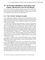
FIGURE
24.17
Predicate
dependency
graph for Figures 24.14
and
24.15.
predicates do
not
have
any incoming edges, since all fact-defined predicates have their
facts stored in a database relation.
The
contents
of a fact-defined predicate

can
be com-
puted
by directly retrieving
the
tuples in
the
corresponding database relation.
The
main
function
of an inference
mechanism
is to compute
the
facts
that
corre-
spond to query predicates.
This
can
be accomplished by generating a relational expres-
sion involving relational operators as SELECT,PROJECT,JOIN, UNION,
and
SET
DIFFERENCE
(with
appropriate provision for dealing
with
safety issues) that,

when
executed, provides
the
query result.
The
query
can
then
be executed by utilizing
the
internal
query process-
ing
and
optimization operations of a relational database
management
system. Whenever
the
inference
mechanism
needs to compute
the
fact set corresponding to a nonrecursive
rule-defined predicate p, it first locates all
the
rules
that
have
p as
their

head.
The
idea is
to compute
the
fact set for
each
such rule
and
then
to apply
the
UNION operation to the
results, since
UNION corresponds to a logical OR operation.
The
dependency graph indi-
cates all predicates q
on
which
each
p depends,
and
since we assume
that
the
predicate is
nonrecursive, we
can
always

determine
a partial order among such predicates q.
Before
computing
the
fact set for p, we first
compute
the
fact sets for all predicates q on which p
depends, based on
their
partial order. For example, if a query involves
the
predicate
under
_40K_supervi
sor,
we must first compute
both
supervisor
and
over
_
40K_emp.
Since
the
latter
two
depend
only on

the
fact-defined predicates employee,
salary,
and super-
vi se, they
can
be
computed
directly from
the
stored database relations.
This
concludes our
introduction
to
deductive databases.
Additional
material may be
found at
the
book
Web
site, where
the
complete
Chapter
25 from
the
third
edition is

available.
This
includes a discussion on algorithms for recursive query processing.
24.5 Summary I
797
24.5 SUMMARY
In this chapter, we introduced database concepts for some of
the
common
features
that
are needed by advanced applications: active databases, temporal databases,
and
spatial
and multimedia databases. It is
important
to
note
that
each
of these topics is very broad
and warrants a complete textbook.
We first introduced
the
topic of active databases,
which
provide additional
functionality for specifying active rules. We introduced
the
event-condition-action

or
ECA model for active databases.
The
rules
can
be automatically triggered by
events
that
occur-such
as a database
update-and
they
can
initiate
certain
actions
that
have
been
specified in
the
rule declaration if
certain
conditions
are true.
Many
commercial packages
already
have
some of

the
functionality provided by active databases in
the
form of
triggers. We discussed
the
different options for specifying rules,
such
as row-level versus
statement-level, before versus after,
and
immediate versus deferred. We gave examples of
row-level triggers in
the
Oracle
commercial system,
and
statement-level rules in
the
STARBURST
experimental
system.
The
syntax for triggers in
the
sQL-99
standard was also
discussed. We briefly discussed some design issues
and
some possible applications for

active databases.
We
then
introduced some of
the
concepts of temporal databases, which permit
the
database system to store a history of changes
and
allow users to query
both
current and past
states of
the
database. We discussed how time is represented
and
distinguished between the
valid time
and
transaction time dimensions. We
then
discussed how valid time, transaction
time,
and
bitemporal relations
can
be implemented using tuple versioning in
the
relational
model, with examples to illustrate

how
updates, inserts,
and
deletes are implemented. We
also showed
how
complex objects
can
be used
to
implement temporal databases using
attribute versioning. We
then
looked at some of
the
querying operations for temporal
relational databases
and
gave a very briefintroduction to
the
TSQL2 language.
We
then
turned
to
spatial
and
multimedia databases. Spatial databases provide
concepts for databases
that

keep track of objects
that
have
spatial characteristics,
and
they require models for representing these spatial characteristics
and
operators for
comparing
and
manipulating
them.
Multimedia databases provide features
that
allow
users to store
and
query different types of multimedia information,
which
includes images
(such as pictures or drawings), video clips (such as movies, news reels, or
home
videos),
audio clips (such as songs,
phone
messages, or speeches),
and
documents (such as books or
articles). We gave a very brief overview of
the

various types of media sources
and
how
multimedia sources may be indexed.
We concluded
the
chapter
with
an
introduction
to deductive databases
and
Datalog.
Review Questions
24.1.
What
are
the
differences
between
row-level
and
statement-level active rules?
24.2.
What
are
the
differences among immediate, deferred,
and
detached

consideration
of active rule conditions?
24.3.
What
are
the
differences among immediate, deferred,
and
detached
execution of
active rule actions?
798 I
Chapter
24 Enhanced
Data
Models for
Advanced
Applications
24.4. Briefly discuss
the
consistency
and
termination
problems
when
designing a set of
active rules.
24.5. Discuss some applications of active databases.
24.6. Discuss
how

time is represented in temporal databases
and
compare
the
different
time dimensions.
24.7.
What
are
the
differences
between
valid time, transaction time,
and
bitemporal
relations?
24.8. Describe how
the
insert, delete,
and
update commands should be implemented on
a valid time relation.
24.9. Describe
how
the
insert, delete,
and
update commands should be implemented on
a bitemporal relation.
24.10. Describe how

the
insert, delete,
and
update commands should be implemented on
a transaction time relation.
24.1 L
What
are
the
main
differences
between
tuple versioning
and
attribute versioning?
24.12. How do spatial databases differ from regular databases?
24.13.
What
are
the
different types of multimedia sources?
24.14. How are multimedia sources indexed for
content-based
retrieval?
Exercises
24.15. Consider
the
COMPANY
database described in Figure 5.6. Using
the

syntax of Oracle
triggers, write active rules to do
the
following:
a.
Whenever
an employee's project assignments are changed,
check
if the total
hours per week
spent
on
the
employee's projects are less
than
30 or greater
than
40; if so, notify
the
employee's direct supervisor.
b.
Whenever
an
EMPLOYEE
is deleted, delete
the
PROJECT
tuples
and
DEPENDENT

tuples
related to
that
employee,
and
if
the
employee is managing a department or
supervising any employees, set
the
MGRSSN
for
that
department
to null and set
the
SUPERSSN
for those employees to nulL
24.16.
Repeat
24.15 but use
the
syntax of STARBURST active rules.
24.17.
Consider
the
relational schema shown in Figure 24.18.
Write
active rules
for

keeping
the
SUM_COMMISSIONS
attribute
of
SALES_PERSON
equal to
the
sum of the
COM-
MISSION
attribute
in SALES for
each
sales person. Your rules should also check if rhe
SALES
~
COMMISSION I
SALESPERSON ID
SUM COMMISSIONS
FIGURE 24.18
Database
schema
for sales
and
salesperson
commissions
in
Exercise
24.17.

SUM_COMMISSIONS
exceeds 100000; if it does, call a procedure NOTIFY_MANAGER(S_ID).
Write
both
statement-level
rules in STARBURST
notation
and
row-level rules in
Oracle.
24.18. Consider
the
UNIVERSITY EER
schema
of Figure 4.10.
Write
some rules (in English)
that
could be
implemented
via active rules
to
enforce some
common
integrity
constraints
that
you
think
are relevant to this application.

24.19. Discuss
which
of
the
updates
that
created
each
of
the
tuples
shown
in Figure 24.9
were applied retroactively
and
which
were applied proactively.
24.20.
Show
how
the
following updates, if applied in sequence, would
change
the
con-
tents
of
the
bitemporal
EMP

_8T
relation in Figure 24.9. For
each
update, state
whether
it is a retroactive or proactive update.
a.
On
2004-03-10,17:30:00,
the
salary of
NARAYAN
is updated to 40000, effective
on 2004-03-01-
b.
On
2003-07-30,08:31:00,
the
salary of SMITH was corrected to show
that
it
should
have
been
entered
as 31000 (instead of 30000 as shown), effective on
2003-06-01-
c.
On
2004-03-18,08:

31: 00,
the
database was changed
to
indicate
that
NARAYAN
was leaving
the
company
(i.e., logically deleted) effective 2004-03-31-
d.
On
2004-04-20,14:
07: 33,
the
database was changed to indicate
the
hiring of
a
new
employee called
JOHNSON,
with
the
tuple
<'
JOHNSON',
'334455667',
1,

NULL> effective on 2004-04-20.
e.
On
2004-04-28,12:
54: 02,
the
database was
changed
to
indicate
that
WONG
was
leaving
the
company (i.e., logically deleted) effective 2004-06-01.
f.
On
2004-05-05,13:
07: 33,
the
database was
changed
to indicate
the
rehiring
of
BROWN,
with
the

same
department
and
supervisor
but
with
salary 35000 effec-
tive
on
2004-05-01-
24.21.
Show
how
the
updates given in Exercise 24.20, if applied in sequence, would
change
the
contents
of
the
valid time
EMP
_VT relation in Figure 24.8.
24.22.
Add
the
following facts to
the
example database in Figure 24.3:
supervise

(ahmad,bob) ,
supervise
(franklin,gwen).
First modify
the
supervisory tree in Figure 24.1b to reflect this change.
Then
mod-
ify
the
diagram in Figure 24.4 showing
the
top-down evaluation of
the
query
superior(james,Y).
24.23.
Consider
the
following set of facts for
the
relation
parent(X,
V), where Y is
the
parent
of
X:
parent(a,aa),
parent(a,ab),

parent(aa,aaa),
parent(aa,aab),
parent(aaa,aaaa),
parent(aaa,aaab).
Consider
the
rules
Exercises I 799
r1:
ancestor(X,Y)
r2:
ancestor(X,Y)
parent(X,Y)
parent(X,Z),
ancestor(Z,Y)
which
define ancestor Yof X as above.
800
I
Chapter
24
Enhanced
Data
Models
for
Advanced
Applications
a.
Show
how

to solve
the
Datalog query
ancestor(aa,X)?
using
the
naive strategy.
Show
your work at
each
step.
b. Show
the
same query by computing only
the
changes in
the
ancestor relation
and
using
that
in rule 2
each
time.
[This question is derived from
Bancilhon
and
Ramakrishnan
(1986).]
24.24.

Consider
a deductive database with
the
following rules:
ancestor(X,Y)
:-
father(X,Y)
ancestor(X,Y)
:-
father(X,Z),
ancestor(Z,Y)
Notice
that
"father(X,Y)"
means
that
Y is
the
father of X;
"ancestor(X,Y)"
means
that
Yis
the
ancestor of
X.
Consider
the
fact base
father(HarrY,Issac)

,
father(Issac,John)
,
father(John,Kurt).
a.
Construct
a model theoretic
interpretation
of
the
above rules using the given
facts.
b. Consider
that
a database
contains
the
above relations
father(X,
V), another
relation
b
rothe
r (X,Y),
and
a
third
relation
bi
rth

(X, B), where B is the birth-
date of person
X.
State
a rule
that
computes
the
first cousins of
the
following
variety:
their
fathers must be brothers.
c.
Show
a complete Datalog program
with
fact-based
and
rule-based literals that
computes
the
following relation: list of pairs of cousins, where
the
first person
is
born
after 1960
and

the
second after 1970. You may use "greater than" as a
built-in predicate.
(Note: Sample facts for brother, birth,
and
person must
also
be shown.)
24.25.
Consider
the
following rules:
reachable(X,Y)
:-
flight(X,Y)
reachable(X,Y)
:-
flight(X,Z),
reachable(Z,Y)
where
reachable
(X, Y) means
that
city Y
can
be reached from city
X,
and
fl
i

ght
(X,Y) means
that
there is a flight to city Yfrom city
X.
a.
Construct
fact predicates
that
describe
the
following:
i. Los Angeles,
New
York, Chicago,
Atlanta,
Frankfurt, Paris, Singapore,
Sydney are cities.
ii.
The
following flights exist: LA
to
NY, NY to
Atlanta,
Atlanta
to Frankfurt,
Frankfurt to
Atlanta,
Frankfurt
to

Singapore,
and
Singapore to
Sydney.
(Note:
No
flight in reverse direction can be automatically assumed.)
b. Is
the
given
data
cyclic?
If
so, in
what
sense?
c.
Construct
a model theoretic
interpretation
(that
is, an interpretation similar
to
the
one
shown in Figure 25.3) of
the
above facts and rules.
d.
Consider

the
query
reachable(Atlanta,Sydney)?
How will this query be executed using naive
and
seminaive evaluation?
List
the
series of steps it will go through.
Selected Bibliography I801
e. Consider
the
following rule-defined predicates:
round-trip-reachable(X,Y)
:-
reachable(X,Y), reachable(Y,X)
duration(X,Y,Z)
Draw a predicate dependency graph for
the
above predicates. (Note:
dura-
t i on(X,Y,Z) means
that
you
can
take a flight from Xto Yin Zhours.)
f. Consider
the
following query:
What

cities are reachable in 12 hours from
Atlanta?
Show
how to express it in Datalog. Assume built-in predicates like
greater-than(X,
V).
Can
this be converted into a relational algebra state-
ment
in a straightforward way?
Why
or why not?
g. Consider
the
predicate
population(X,
Y)
where Y is
the
population of city
X.
Consider
the
following query: List all possible bindings of
the
predicate
pai r (X,V), where Yis a city
that
can
be reached in two flights from city

X,
which
has over 1 million people. Show this query in Datalog, Draw a corre-
sponding query tree in relational algebraic terms.
Selected Bibliography
The
book by Zaniolo et al. (1997) consists of several parts,
each
describing an advanced
database
concept
such as active, temporal,
and
spatial/text/multimedia databases. Widom
and Ceri (1996)
and
Ceri
and
Fraternali (1997) focus
on
active database concepts and
systems. Snodgrass et al. (1995) describe
the
TSQL2 language and
data
model. Khoshafian
and Baker (1996), Faloutsos (1996),
and
Subrahmanian
(1998) describe multimedia

database concepts. Tansel et al. (1992) is a collection of chapters on temporal databases.
STARBURST rules are described in
Widom
and
Finkelstein (1990). Early work on
active databases includes
the
HiPAC
project, discussed in Chakravarthy et al. (1989) and
Chakravarthy (1990). A glossary for temporal databases is given in Jensen et al. (1994).
Snodgrass (1987) focuses
on
TQuel,
an early temporal query language.
Temporal normalization is
defined in N avathe
and
Ahmed
(1989).
Paton
(1999) and
Paton
and
Diaz (1999) survey active databases.
Chakravarthy
et al. (1994) describe
SENTINEL,
and
object-based active systems. Lee et al. (1998) discuss time series
management.

The
early developments of
the
logic and database approach are surveyed by Gallaire
et al. (1984). Reiter (1984) provides a reconstruction of relational database theory, while
Levesque (1984) provides a discussion of incomplete knowledge in light of logic. Gallaire
and
Minker
(1978) provide an early book
on
this topic. A detailed
treatment
oflogic and
databases appears in
Ullman
(1989, vol. 2), and there is a related chapter in Volume 1
(1988). Ceri,
Gottlob,
and
Tanca
(1990) present a comprehensive yet concise
treatment
of logic
and
databases. Das (1992) is a comprehensive book
on
deductive databases and
logic programming.
The
early history of Datalog is covered in Maier

and
Warren (1988).
Clocksin
and
Mellish (1994) is
an
excellent reference
on
Prolog language.
Aho
and
Ullman
(1979) provide an early algorithm for dealing with recursive
queries, using
the
least fixed-point operator. Bancilhon and Ramakrishnan (1986) give an
excellent
and
detailed description of
the
approaches to recursive query processing,
with
detailed examples of
the
naive and seminaive approaches. Excellent survey articles
on
802 I Chapter 24 Enhanced Data Models for Advanced Applications
deductive databases
and
recursive query processing include

Warren
(1992) and
Ramakrishnan and
Ullman
(1993). A complete description of
the
seminaive approach
based on relational algebra is given in Bancilhon (1985).
Other
approaches to recursive
query processing include
the
recursive query/subquery strategy of Vieille (1986), which is
a
top-down interpreted strategy,
and
the
Henschen-
Naqvi (1984) top-down compiled
iterative strategy. Balbin and Rao (1987) discuss an extension of
the
seminaive
differential approach for multiple predicates.
The
original paper on magic sets is by Bancilhon et at. (1986). Beeri and
Ramakrishnan (1987)
extend
it. Mumick et at. (1990) show
the
applicability of

magic
sets to nonrecursive nested
SQL
queries.
Other
approaches to optimizing rules without
rewriting
them
appear in Vieille (1986, 1987). Kifer
and
Lozinskii (1986) propose a
different technique. Bry (1990) discusses how
the
top-down and bottom-up approaches
can
be reconciled.
Whang
and
Navathe
(1992) describe an
extended
disjunctive normal
form
technique
to deal with recursion in relational algebra expressions for providing an
expert system interface over a relational
DBMS.
Chang
(1981) describes
an

early system for combining deductive rules with relational
databases.
The
LOL
system prototype is described in
Chimenti
et at. (1990).
Krishnamurthy and
Naqvi
(1989) introduce
the
"choice"
notion
in LDL. Zaniolo (1988)
discusses
the
language issues for
the
LOL
system. A language overview of
CORAL
is
provided in Ramakrishnan et at. (1992),
and
the
implementation is described in
Ramakrishnan et at. (1993).
An
extension to support object-oriented features, called
CORAL++, is described in Srivastava et at. (1993).

Ullman
(1985) provides
the
basis for
the
NAIL!
system,
which
is described in Morris et at. (1987). Phipps et at. (1991) describe
the
GLUE-NAIL!
deductive database system.
Zaniolo (1990) reviews
the
theoretical background and
the
practical importance of
deductive databases. Nicolas (1997) gives an excellent history of
the
developments
leading up to
OOOOs.
Falcone et at. (1997) survey
the
0000
landscape. References on the
VALIDITY
system include Friesen et at. (1995), Vieille (1997), and Dietrich et at. (1999).
Distributed Databases
and Client-Server

Architectures
In
this
chapter
we
tum
our
attention
to distributed databases
(DDBs),
distributed data-
base
management
systems
(DDBMSs),
and
how
the
client-server architecture is used as a
platform for database
application
development.
The
DDB
technology emerged as a merger
of two technologies: (1) database technology,
and
(2)
network
and

data
communication
technology.
The
latter
has
made
tremendous strides in terms of wired
and
wireless
technologies-from
satellite
and
cellular
communications
and
Metropolitan
Area
Net-
works (MANs) to
the
standardization of protocols like
Ethernet,
TCPjIP,
and
the
Asyn-
chronous Transfer
Mode
(ATM) as well as

the
explosion of
the
Internet.
While
early
databases
moved
toward centralization
and
resulted in
monolithic
gigantic databases in
the seventies
and
early eighties,
the
trend
reversed toward more decentralization
and
autonomy of processing in
the
late eighties.
With
advances in distributed processing
and
distributed
computing
that
occurred in

the
operating
systems arena,
the
database
research
community
did considerable work to address
the
issues of
data
distribution, dis-
tributed query
and
transaction
processing, distributed database rnetadata management,
and
other
topics,
and
developed
many
research prototypes. However, a full-scale compre-
hensive
DDBMS
that
implements
the
functionality
and

techniques proposed in
DDB
research
never
emerged as a commercially viable product. Most major vendors redirected
their efforts from developing a "pure"
DDBMS
product
into
developing systems based
on
client-server, or toward developing technologies for accessing distributed heterogeneous
data sources.
803
804
I Chapter 25 Distributed Databases
and
Client-Server Architectures
Organizations, however,
have
been
very interested in
the
decentralization
of
processing
(at
the
system level) while achieving an integmtion of
the

information
resources
(at
the logical level)
within
their
geographically distributed systems of
databases, applications,
and
users.
Coupled
with
the
advances in communications, there
is
now
a general
endorsement
of
the
client-server approach to application development,
which
assumes many of
the
DDB issues.
In this
chapter
we discuss
both
distributed databases

and
client-server architectures.'
in
the
development
of database technology
that
is closely tied to advances in
communications
and
network technology. Details of
the
latter
are outside our scope; the
reader is referred to a series of texts on
data
communications
and
networking (see the
Selected Bibliography at
the
end
of this chapter).
Section
25.1
introduces distributed database management and related concepts.
Detailed issuesof distributed database design, involving fragmenting of
data
and
distributing

it over multiple sites with possible replication, are discussed in Section
25.2.
Section
25.3
introduces different types of distributed database systems, including federated and
multidatabase systems
and
highlights
the
problems of heterogeneity and the needs of
autonomy in federated database systems, which will dominate for years to come. Sections
25.4
and
25.5
introduce distributed database query
and
transaction processing techniques,
respectively. Section
25.6discusses how
the
client-server architectural concepts are
related
to distributed databases. Section
25.7
elaborates on future issues in client-server
architectures. Section
25.8discusses distributed database features of
the
Oracle
RDBMS.

For a short introduction to
the
topic, only sections 25.1,25.3,
and
25.6may be
covered.
25.1 DISTRIBUTED
DATABASE
CONCEPTS
Distributed databases bring the advantages of distributed computing to the database
man-
agement domain. A distributed computing system consists of a number of processing
ele-
ments,
not
necessarily homogeneous,
that
are interconnected by a computer network, and
that
cooperate in performing certain assigned tasks. As a general goal, distributed
comput-
ing systems partition a big, unmanageable problem into smaller pieces and solve it
effi-
ciently in a coordinated manner.
The
economic viability of this approach stems from
two
reasons:
(l)
more computer power is harnessed to solve a complex task, and (2) each auton-

omous processing element
can
be managed independently
and
develop its own applications.
We
can
define a
distributed
database (OOB) as a collection of multiple
logically
interrelated databases distributed over a
computer
network,
and
a
distributed
database
management
system (OOBMS) as a software system
that
manages a distributed database
while making
the
distribution transparent to
the
user.
l
A collection of files stored at
different nodes of a

network
and
the
maintaining of interrelationships among them via
hyperlinks has become a
common
organization on
the
Internet,
with
files of Web
pages.
1.
The
reader should review
the
introduction
to client-server architecture in
Section
2.5.
2.
This
definition
and
some of the discussion in this
section
are based
on
Ozsu and
Valduriez

(1999).
25.1 Distributed Database Concepts I805
The
common
functions of database
management,
including uniform query processing
and
transaction
processing, do not apply to this scenario yet.
The
technology is, however,
moving in a direction such
that
distributed World
Wide
Web
(WWW)
databases will
become a reality in
the
near
future. We shall discuss issues of accessing databases
on
the
Web in
Chapter
26.
None
of those qualifies as DDB by

the
definition given earlier.
25.1.1 Parallel Versus Distributed Technology
Turning
our
attention
to parallel system architectures,
there
are two
main
types of multi-
processor system architectures
that
are commonplace:
•
Shared
memory
(tightly
coupled)
architecture: Multiple processors share secondary
(disk) storage
and
also share primary memory.
•
Shared
disk
(loosely
coupled)
architecture:
Multiple processors share secondary (disk)

storage
but
each
has
their
own
primary memory.
These
architectures
enable
processors to
communicate
without
the
overhead
of
exchanging
messages
over
a network.:' Database
management
systems
developed
using
the
above types of
architectures
are
termed
parallel

database
management
systems
rather
than
DDBMS, since
they
utilize parallel processor technology.
Another
type of
multiprocessor
architecture
is called
shared
nothing
architecture.
In this
architecture,
every processor
has
its
own
primary
and
secondary (disk) memory,
no
common
memory
exists,
and

the
processors
communicate
over
a high-speed
interconnection
network
(bus or
switch).
Although
the
shared
nothing
architecture
resembles a
distributed
database
computing
environment,
major
differences exist in
the
mode
of
operation.
In
shared
nothing
multiprocessor systems,
there

is symmetry
and
homogeneity
of nodes;
this is
not
true
of
the
distributed
database
environment
where
heterogeneity
of
hardware
and
operating
system at
each
node
is very
common.
Shared
nothing
architecture
is also
considered
as an
environment

for parallel databases. Figure 25.1
contrasts
these
different
architectures.
25.1.2 Advantages
of
Distributed Databases
Distributed database
management
has
been
proposed for various reasons ranging from
organizational decentralization
and
economical processing to greater autonomy. We high-
light some of these advantages here.
1. Management of distributed data with different
levels
of
transparency:
Ideally, a DBMS
should be
distribution
transparent
in
the
sense of hiding
the
details of where

each
file (table, relation) is physically stored
within
the
system.
Consider
the
company database in Figure 5.5
that
we
have
been
discussing
throughout
the





3. If
both
primary
and
secondary memories are shared,
the
architecture is also
known
as
shared

everything
architecture.
806
I Chapter 25 Distributed Databases
and
Client-Server Architectures
(a)
Computer System 1
Switch
Computer System 2
Computer System n
(b)
Site
(San Francisco)
Central
Site
(Chicago)
Site
(New York)
Site
(Los Angeles)
Communications
Network
Site
(Atlanta)
(c)
Communications
Network
fIGURE 25.1
Some

different
database
system architectures. (a) Shared nothing
architecture. (b) A networked architecture with a centralized
database
at
one
of the
sites. (c) A truly distributed
database
architecture.
25.1 Distributed
Database
Concepts I
807
book.
The
EMPLOYEE,
PROJECT,
and
WORKS_ON
tables may be fragmented horizontally
(that
is,
into
sets of rows, as we shall discuss in
Section
25.2)
and
stored

with
pos-
sible replication as
shown
in Figure 25.2.
The
following types of transparencies
are possible:
• Distribution or network transparency:
This
refers to freedom for
the
user from
the
operational details of
the
network.
It
may be divided
into
location transparency
and
naming
transparency.
Location
transparency
refers to
the
fact
that

the
command
used to perform a task is
independent
of
the
location
of
data
and
the
location of
the
system where
the
command
was issued.
Naming
transparency
implies
that
once
a
name
is specified,
the
named
objects
can
be accessed unam-

biguously
without
additional specification.
•
Replication
transparency: As we show in Figure 25.2, copies of
data
may be stored
at multiple sites for
better
availability, performance,
and
reliability.
Replication
transparency makes
the
user unaware of
the
existence of copies.
• Fragmentation transparency: Two types
offragmentation
are possible.
Horizontal
fragmentation
distributes a
relation
into
sets of tuples (rows). Vertical fragmen-
tation
distributes a relation

into
subrelations where
each
subrelation is defined
by a subset of
the
columns of
the
original relation. A global query by
the
user
must be transformed
into
several fragment queries. Fragmentation transparency
makes
the
user unaware of
the
existence of fragments.
EMPLOYEES-San Francisco
and Los Angeles
PROJECTs-
San Francisco
WORKS_ON-San Francisco
Employees
San Francisco
Los Angeles
EMPLOYEES-los Angeles
PROJECTS- Los Angeles and
San Francisco

WORKs_ON-Los
Angeles
Employees
EMPLOYEES-All
PROJECTS- All
WORKS_ON-AII
Communications
Network
New York
Atlanta
EMPLOYEES-NewYork
PROJECTS- All
WORKS_ON-
NewYork
Employees
EMPLOYEES-Atlanta
PROJECTS- Atlanta
WORKS_ON-Atlanta
Employees
FIGURE
25.2
Data
distribution
and
replication
among
distributed
databases
808
I Chapter 25 Distributed Databases

and
Client-Server Architectures
2.
Increased
reliability
and
availability:
These
are two of
the
most
common
potential
advantages cited for distributed databases. Reliability is broadly defined as the
probability
that
a system is
running
(not
down) at a
certain
time point, whereas
availability is
the
probability
that
the
system is continuously available during a
time
interval.

When
the
data
and
DBMSsoftware are distributed over several sites,
one
site may fail while
other
sites
continue
to operate.
Only
the
data
and
software
that
exist at
the
failed site
cannot
be accessed.
This
improves
both
reliability and
availability.
Further
improvement
is achieved by judiciously

replicating
data and
software at more
than
one
site. In a centralized system, failure at a single site
makes
the
whole system unavailable to all users. In a distributed database, someof
the
data
may be unreachable,
but
users may still be able
to
access
other
parts of
the
database.
3.
Improved
performance:
A distributed DBMSfragments
the
database by keeping the
data
closer to where it is
needed
most.

Data
localization reduces
the
contention
for
CPU
and
I/O services
and
simultaneously reduces access delays involved in
wide area networks.
When
a large database is distributed over multiple
sites,
smaller databases exist at
each
site. As a result, local queries
and
transactions
accessing
data
at a single site
have
better
performance because of
the
smaller
local
databases. In addition,
each

site has a smaller
number
of transactions executing
than
if all transactions are submitted to a single centralized database.
Moreover,
interquery
and
intraquery parallelism
can
be achieved by executing multiple
que-
ries at different sites, or by breaking up a query
into
a
number
of subqueries that
execute in parallel.
This
contributes to improved performance.
4.
Easier
expansion:
In a distributed
environment,
expansion of
the
system in
terms
of adding more data, increasing database sizes, or adding more processors is much

easier.
The
transparencies we discussed in (1) above lead to a compromise between easeof
use
and
the
overhead cost of providing transparency. Total transparency provides the
global user
with
a view of
the
entire
DDBS as if it is a single centralized
system.
Transparency is provided as a
complement
to
autonomy,
which
gives
the
users tighter
control
over
their
own local databases. Transparency features may be implemented as a
part
of
the
user language,

which
may translate
the
required services into appropriate
operations. In addition, transparency impacts
the
features
that
must be provided by the
operating system
and
the
DBMS.
25.1.3
Additional Functions of Distributed Databases
Distribution leads to increased complexity in
the
system design
and
implementation.
To
achieve
the
potential
advantages listed previously,
the
DDBMS
software must be able to
provide
the

following functions in addition to those of a centralized
DBMS:
•
Keeping
track
of data:
The
ability to keep track of
the
data
distribution, fragmenta-
tion,
and
replication by expanding
the
DDBMS catalog.
25.1 Distributed Database Concepts I 809
• Distributed query
processing:
The
ability to access
remote
sites
and
transmit
queries
and
data
among
the

various sites via a
communication
network.
• Distributed transaction management:
The
ability to devise
execution
strategies for
que'
ries
and
transactions
that
access
data
from more
than
one
site
and
to synchronize
the
access to distributed
data
and
maintain
integrity of
the
overall database.
•

Replicated
data management:
The
ability to decide
which
copy of a replicated
data
item
to
access
and
to
maintain
the
consistency of copies of a replicated
data
item.
• Distributed
database
recovery:
The
ability
to
recover from individual site crashes
and
from
new
types of failures such as
the
failure of a

communication
links.
• Security: Distributed transactions must be
executed
with
the
proper
management
of
the
security of
the
data
and
the
authorization/access privileges of users.
• Distributed
directory
(catalog)
management: A directory
contains
information (meta-
data)
about
data
in
the
database.
The
directory may be global for

the
entire
DDB, or
local for
each
site.
The
placement
and
distribution of
the
directory are design
and
policy issues.
These
functions themselves increase
the
complexity of a
DDBMS
over a centralized
DBMS. Before we
can
realize
the
full
potential
advantages of distribution, we must find
satisfactory solutions to these design issues
and
problems. Including all this additional

functionality is
hard
to
accomplish,
and
finding
optimal
solutions is a step beyond that.
At
the
physical
hardware
level,
the
following
main
factors distinguish a
DDBMS
from
a centralized system:
•
There
are multiple computers, called sites or nodes.
•
These
sites must be
connected
by some type of
communication
network

to transmit
data
and
commands
among
sites, as shown in Figure 25.1c.
The
sites may all be located in physical
proximity-say,
within
the
same building or
group of
adjacent
buildings-and
connected
via a local
area
network,
or they may be
geographically distributed over large distances
and
connected
via a
long-haul
or wide
area
network.
Local area networks typically use cables, whereas long-haul networks use
telephone

lines or satellites.
It
is also possible to use a
combination
of
the
two types of
networks.
Networks
may
have
different topologies
that
define
the
direct
communication
paths
among
sites.
The
type
and
topology of
the
network
used may
have
a significant
effect

on
performance
and
hence
on
the
strategies for
distributed
query processing
and
distributed
database
design. For
high-level
architectural
issues, however, it does
not
matter
which
type of
network
is used; it
only
matters
that
each
site is able to
communicate,
directly or indirectly,
with

every
other
site. For
the
remainder
of this
chapter, we assume
that
some type of
communication
network
exists
among
sites,
regardless of
the
particular
topology. We will
not
address
any
network
specific issues,
although
it is
important
to
understand
that
for

an
efficient
operation
of a DDBS,
network
design
and
performance
issues are very critical.
810 I
Chapter
25 Distributed Databases
and
Client-Server Architectures
25.2 DATA FRAGMENTATION,
REPLICATION,
AND
ALLOCATION
TECHNIQUES
FOR
DISTRIBUTED
DATABASE
DESIGN
In this section we discuss techniques
that
are used to break up
the
database
into
logical

units, called fragments,
which
may be assigned for storage at
the
various sites. We also
discuss
the
use of
data
replication,
which
permits
certain
data
to be stored in more than
one
site,
and
the
process of allocating
fragments-or
replicas of
fragments-for
storage at
the
various sites.
These
techniques are used during
the
process of

distributed
database
design.
The
information
concerning
data
fragmentation, allocation,
and
replication is
stored in a global
directory
that
is accessed by
the
DDBSapplications as needed.
25.2.1 Data Fragmentation
In a DDB, decisions must be made regarding
which
site should be used to store which por-
tions of
the
database. For now, we will assume
that
there
is no
replication;
that
is, each
relation-or

portion
of a
relation-is
to be stored at only
one
site. We discuss replication
and
its effects later in this section. We also use
the
terminology of relational
databases-
similar concepts apply to
other
data
models. We assume
that
we are starting
with
a
rela-
tional
database schema
and
must decide
on
how
to distribute
the
relations over the vari-
ous sites. To illustrate our discussion, we use

the
relational database schema in Figure
5.5.
Before we decide on
how
to distribute
the
data, we must
determine
the
logical
units
of
the
database
that
are to be distributed.
The
simplest logical units are
the
relations
themselves;
that
is,
each
whole
relation is to be stored at a particular site. In our example,
we must decide on a site to store
each
of

the
relations
EMPLOYEE,
DEPARTMENT,
PROJECT,
WORKS_ON,
and
DEPENDENT
of Figure 5.5. In many cases, however, a relation
can
be divided into smaller
logical units for distribution. For example, consider
the
company database shown in
Figure
5.6,
and
assume
there
are three
computer
sites-one
for
each
department
in the
cornpanv," We may
want
to store
the

database information relating to
each
department at
the
computer
site for
that
department.
A
technique
called
horizontal
fragmentation
can be
used to
partition
each
relation by department.
Horizontal
Fragmentation. A horizontal fragment of a relation is a subset of the
tuples in
that
relation.
The
tuples
that
belong
to
the
horizontal fragment are specifiedbya

condition
on
one
or more attributes of
the
relation. Often, only a single attribute is
involved. For example, we may define three horizontal fragments on
the
EMPLOYEE
relation of
Figure
5.6with
the
following conditions:
(DNO
= 5),
(DNO
= 4), and
(DNO
=
l)-each
fragment
contains
the
EMPLOYEE
tuples working for a particular department. Similarly, we may
define
three horizontal fragments for
the
PROJECT

relation, with the conditions
(DNUM
= 5),
(DNUM
= 4),
4.
Of
course, in an actual situation, there will be many more tuples in
the
relations
than
those
shown in Figure 5.6.
25.2 Data Fragmentation, Replication, and
Allocation
Techniques I 811
and
(DNUM
= I
) each
fragment contains the
PROJ
ECT
tuples controlled by a particular
department.
Horizontal
fragmentation divides a relation "horizontally" by grouping rows to
create subsets of tuples, where
each
subset has a certain logical meaning. These fragments

can
then
be assigned to different sites in
the
distributed system.
Derived
horizontal
fragmentation applies
the
partitioning of a primary relation
(DEPARTMENT
in our example) to
other
secondary relations
(EMPLOYEE
and
PROJECT
in our example), which are related to
the
primary via a foreign key.
This
way, related data between
the
primary
and
the
secondary
relations gets fragmented in
the
same way.

Vertical
Fragmentation.
Each site may
not
need
all
the
attributes of a relation,
which
would indicate
the
need
for a different type of fragmentation. Vertical
fragmentation
divides a relation "vertically" by columns. A
vertical
fragment
of a
relation keeps only
certain
attributes of
the
relation. For example, we may
want
to
fragment
the
EMPLOYEE
relation
into

two vertical fragments.
The
first fragment includes
personal information-NAME,
BDATE,
ADDRESS,
and
sEx-and
the
second includes work-related
informarion-s-sss,
SALARY,
SUPERSSN,
DNO.
This
vertical fragmentation is
not
quite proper
because, if
the
two fragments are stored separately, we
cannot
put
the
original employee
tuples back together, since
there
is no common attribute
between
the

two fragments.
It
is
necessary
to
include
the
primary key or some
candidate
key
attribute
in every vertical
fragment so
that
the
full
relation
can
be reconstructed from
the
fragments.
Hence,
we
must add
the
SSN
attribute to
the
personal information fragment.
Notice

that
each
horizontal fragment
on
a relation R
can
be specified by a (JCi(R)
operation in
the
relational algebra. A set of horizontal fragments whose conditions
CI,
C2,

,
Cn
include all
the
tuples in
R-that
is, every tuple in R satisfies
(CI
ORC2 OR

OR
Cn)-is
called a complete
horizontal
fragmentation of R. In many cases a complete
horizontal fragmentation is also disjoint;
that

is,
no
tuple in R satisfies
(Ci
AND
Cj)
for any
i
*"
j.
Our
two earlier examples of horizontal fragmentation for
the
EMPLOYEE
and
PROJECT
relations were
both
complete
and
disjoint. To reconstruct
the
relation R from a
complete
horizontal fragmentation, we
need
to apply
the
UNIONoperation to
the

fragments.
A vertical fragment
on
a relation R
can
be specified by a 7TLi (R)
operation
in
the
relational algebra. A set of vertical fragments whose projection lists L1, L2,

, Ln
include all
the
attributes in R
but
share only
the
primary key
attribute
of R is called a
complete
vertical
fragmentation
ofR.
In this case
the
projection lists satisfy
the
following

two conditions:
• L1 U L2 U

U Ln = ATTRS(R).
• Li n Lj = PK(R) for any i
*-
j,
where ATTRS(R) is
the
set of attributes of
Rand
PK(R) is
the
primary key of R.
To reconstruct
the
relation
R from a
complete
vertical fragmentation, we apply
the
OUTER
UNION
operation
to
the
vertical fragments (assuming
no
horizontal fragmentation
is used).

Notice
that
we could also apply a
FULL
OUTER
JOIN
operation
and
get
the
same
result for a complete vertical fragmentation,
even
when
some horizontal fragmentation
may also
have
been
applied.
The
two vertical fragments of
the
EMPLDYEE
relation
with
projection lists LI =
{SSN,
NAME,
BDATE,
ADDRESS,

SEX}
and
L2 =
{SSN,
SALARY,
SUPERSSN,
DNO}
constitute
a
complete
vertical fragmentation of
EMPLOYEE.
812 I
Chapter
25 Distributed
Databases
and
Client-Server Architectures
Two horizontal fragments
that
are neither complete
nor
disjoint are those defined on the
EMPLOYEE
relation of Figure 5.5 by
the
conditions
(SALARY>
50000) and
(DNO

= 4); they maynot
include all
EMPLOYEE
tuples, and they may include common tuples. Two vertical fragments that
are
not
complete are those defined by the attribute lists L1 =
{NAME,
ADDRESS}
and L2 = {SSN,
NAME,
SALARY};
these lists violate
both
conditions of a complete vertical fragmentation.
Mixed
(Hybrid)
Fragmentation
We
can
intermix
the
two types of fragmentation,
yielding a mixed
fragmentation.
For example, we may
combine
the
horizontal and
vertical fragmentations of

the
EMPLOYEE
relation given earlier
into
a mixed fragmentation
that
includes six fragments. In this case
the
original relation
can
be reconstructed by
applying
UNION
and
OUTER
UNION
(or
OUTER
JOIN)
operations in
the
appropriate order.
In general, a
fragment
of a
relation
R
can
be specified by a
SELECT-PROJECT

combination
of operations
TIL(udR)).
If C =
TRUE
(that
is, all tuples are selected)
and
L
-=1=
ATTRS(R),
we get a vertical fragment,
and
if e
-=1=
TRUE
and
L = ATTRS(R), we get a horizontal
fragment. Finally,
ifC
-=1=
TRUE
and
L
-=1=
ATTRS(R), we get a mixed fragment.
Notice
that
a
relation

can
itself be considered a fragment
with
e =
TRUE
and
L = ATTRS(R). In the
following discussion,
the
term
fragment is used
to
refer to a relation or to any of the
preceding types of fragments.
A
fragmentation
schema
of a database is a definition of a set of fragments that
includes
allattributes
and
tuples in
the
database
and
satisfies
the
condition
that
the whole

database
can
be reconstructed from
the
fragments by applying some sequence of
OUTER
UNION
(or
OUTER
JOIN)
and
UNION
operations. It is also sometimes
useful-although
not
necessary-to
have
all
the
fragments be disjoint
except
for
the
repetition
of primary
keys
among vertical (or mixed) fragments. In
the
latter case, all replication
and

distribution of
fragments is clearly specified at a subsequent stage, separately from fragmentation.
An
allocation
schema
describes
the
allocation of fragments to sites of
the
DDBS;
hence,
it is a mapping
that
specifies for
each
fragment
the
sitets) at
which
it is stored. Ifa
fragment is stored at more
than
one
site, it is said
to
be replicated. We discuss data
replication
and
allocation next.
25.2.2 Data Replication and Allocation

Replication is useful in improving the availability of data.
The
most extreme case is
replica-
tion of the
whole
database
at every site in
the
distributed system, thus creating a fully replicated
distributed database. This
can
improve availability remarkably because the system can con-
tinue to operate as long as at least one site is up. It also improves performance of retrieval
for
global queries, because
the
result of such a query can be obtained locally from
anyone
site;
hence, a retrieval query can be processed at the local site where it is submitted, if that site
includes a server module.
The
disadvantage of full replication is
that
it can slow down update
operations drastically, since a single logical update must be performed on every copy of the
database to keep the copies consistent. This is especially true if many copies of the database
exist. Full replication makes
the

concurrency control and recovery techniques more expensive
than
they would be if there were no replication, as we shall see in Section 25.5.
The
other
extreme from full replication involves having no
replication-that
is,
each
fragment is stored at exactly
one
site. In this case all fragments must be disjoint,
25.2 Data Fragmentation, Replication, and
Allocation
Techniques I 813
except for
the
repetition of primary keys among vertical (or mixed) fragments.
This
is also
called
nonredundant
allocation.
Between these two extremes, we
have
a wide spectrum of
partial
replication of
the
data-that

is, some fragments of
the
database may be replicated whereas others may not.
The
number
of copies of
each
fragment
can
range from
one
up to
the
total
number
of sites
in
the
distributed system. A special case of partial replication is occurring heavily in
applications where mobile
workers-such
as sales forces, financial planners,
and
claims
adjustors-carry
partially replicated databases with
them
on
laptops and personal digital
assistants and synchronize

them
periodically with
the
server database.i A description of
the
replication of fragments is sometimes called a replication schema.
Each
fragment-or
each
copy of a
fragment-must
be assigned to a particular site in
the
distributed system.
This
process is called
data
distribution
(or
data
allocation).
The
choice of sites
and
the
degree of replication depend
on
the
performance
and

availability
goals of
the
system
and
on
the
types
and
frequencies of transactions submitted at
each
site. For example, if
high
availability is required
and
transactions
can
be submitted at any
site and if most transactions are retrieval only, a fully replicated database is a good choice.
However, if
certain
transactions
that
access particular parts of
the
database are mostly
submitted at a particular site,
the
corresponding set of fragments
can

be allocated at
that
site only.
Data
that
is accessed at multiple sites
can
be replicated at those sites. If many
updates are performed, it may be useful to limit replication. Finding an optimal or
even
a
good solution to distributed
data
allocation is a complex optimization problem.
25.2.3 Example of Fragmentation, Allocation,
and Replication
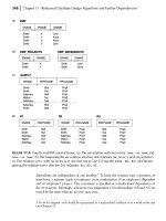
We now consider
an
example of fragmenting and distributing
the
company database of Fig-
ures 5.5 and 5.6. Suppose
that
the
company has three computer
sites one
for each current
department. Sites 2 and 3 are for departments 5 and 4, respectively.
At
each of these sites,

we expect frequent access to
the
EMPLOYEE
and
PROJECT
information for
the
employees who
work
in thatdepartment and
the
projects
controlled
bythat
department.
Further, we assume
that
these sites mainly access
the
NAME,
SSN,
SALARY,
and
SUPERSSN
attributes of
EMPLOYEE.
Site 1 is
used by company headquarters and accesses all employee and project information regularly,
in addition to keeping track of
DEPENDENT

information for insurance purposes.
According to these requirements,
the
whole database of Figure 5.6
can
be stored at
site
1. To determine
the
fragments to be replicated at sites 2
and
3, we
can
first
horizontally fragment
DEPARTMENT
by its key
DNUMBER.
We
then
apply derived fragmentation
to
the
relations
EMPLOYEE,
PROJECT,
and
DEPT_LOCATIONS
relations based on
their

foreign keys
for
department
number-called
DNO,
DNUM,
and
DNUMBER,
respectively, in Figure 5.5. We
can
then
vertically fragment
the
resulting
EMPLOYEE
fragments to include only
the
attributes
{NAME, SSN, SALARY,
SUPERSSN,
DNO}. Figure 25.3 shows
the
mixed fragments
EMPD5
and
EMPD4,
which
include
the
EMPLOYEE

tuples satisfying
the
conditions
DNO
= 5 and
DNO
= 4,
5. For a scalable approach to synchronize partially replicated databases, see Mahajan et al. (1998).
814 I Chapter 25 Distributed Databases and Client-Server Architectures
(a)
I
EMPD5
FNAME
MINIT
LNAME
SSN
SALARY
SUPERSSN
DNO
-
John
B
Smith
123456789
30000 333445555
5
Franklin
T Wcq;
333445555
40000

888665555
5
Ramesh
K
Naravan
666884444
38000 333445555
5
Jcryce
A
English
453453453
25000 333445555
5
DNAME
MGRSTARTDATE
1988-05-22
I
DEP5_LOCS
DNUMBER
LOCATION
5
Bellaire
5
SugaJ1and
5 Houston
J
WORKS
ONS
ESSN PNO

HOURS
123456789 1
32.5
123456789 2
7.5
666884444
3
40.0
453453453
1 20.0
453453453
2
20.0
333445555 2
10.0
333445555
3
10.0
333445555
10
10.0
333445555
20
10.0
!
PROJS5
PNAME
PNUMBER
PLOCATION
DNUM

ProductX
1
Bellaire
5
ProductY
2
Sugarland
5
ProductZ
3
Houston
5
Data at Site 2
(b)
I
EMPD4
FNAME
MINIT
LNAME
SSN
SALARY
SUPERSSN
DNO
-
AIic:ia
J
Zelaya
999887777 25000
987654321
4

Jemifer
S
Wallace
987654321
43000
888665555
4
Ahmad
V
Jabbar
987987987 25000
987654321
4
DNAME
Administration
MGRSTARTDATE
1995-01-01
IDEP4 lOCS I
DNU~BER
I
=ON
I
I
WORKS_ON4
ESSN
PNO
HOURS
333445555 10
10.0
999887777 30

30.0
999887777
10 10.0
987987987
10
35.0
987987987 30
5.0
987654321
30
20.0
987654321 20 15.0
I
PROJS4
PNAME
PNUMBER
PLOCATION
DNUM
Computerization
10
Stafford
4
Newbenefits
30
Staffold
4
Data at Site 3
FIGURE
25.3
Allocation

of
fragments to sites. (a) Relation fragments at site 2 corresponding to
department 5. (b) Relation fragments at site 3 corresponding to department 4.
respectively.
The
horizontal fragments of
PROJECT,
DEPARTMENT,
and
DEPCLOCATIONS are
similarly fragmented by
department
number.
All
these
fragments-stored
at sites 2 and
3-are
replicated because they are also stored at
the
headquarters site 1.
We must now fragment
the
WORKS_ON
relation
and
decide which fragments of
WORKS_ON
to store at sites 2
and

3. We are confronted
with
the
problem
that
no attribute of
WORKS_ON
25.3 Types of Distributed
Database
Systems I815
directly indicates
the
department
to
which
each
tuple belongs. In fact,
each
tuple in
WORKS_
ON
relates an employee e to a project p. We could fragment
WORKS_ON
based on
the
department
d in
which
e works or based
on

the
department
d'
that
controls p.
Fragmentation becomes easy if we have a constraint stating
that
d =
d'
for all
WORKS_ON
tuples-that
is, if employees
can
work only on projects controlled by
the
department
they
work for. However, there is no such constraint in our database of Figure 5.6. For example,
the
WORKS_ON
tuple
<333445555,
10,
10.0>
relates an employee who works for
department
5
with
a project controlled by

department
4. In this case we could fragment
WORKS_ON
based
on
the
department
in which
the
employee works
(which
is expressed by
the
condition
C)
and
then
fragment further based
on
the
department
that
controls
the
projects
that
employee is working
on,
as
shown

in Figure 25.4.
In Figure 25.4,
the
union
of fragments
01,
02,
and
03
gives all
WORKS_ON
tuples for
employees
who
work for
department
5. Similarly,
the
union
of fragments
04,
OS,
and
06
gives all
WORKS_ON
tuples for employees who work for
department
4.
On

the
other
hand,
the
union
of fragments
01,
04,
and
07
gives all
WORKS_ON
tuples for projects controlled by
department
5.
The
condition
for
each
of
the
fragments
01
through
09
is shown in Figure
25.4.
The
relations
that

represent M:N relationships, such as
WORKS_ON,
often
have
several
possible logical fragmentations. In our distribution of Figure 25.3, we choose to include all
fragments
that
can
be joined to
either
an
EMPLOYEE
tuple or a
PROJECT
tuple at sites 2
and
3.
Hence, we place
the
union
of fragments
01,
02, 03, 04,
and
07
at site 2
and
the
union

of
fragments
04,
OS,
06, 02,
and
08
at site 3.
Notice
that
fragments
02
and
04
are
replicated at
both
sites.
This
allocation strategy permits
the
join
between
the
local
EMPLOYEE
or
PROJECT
fragments at site 2 or site 3
and

the
local
WORKS_ON
fragment
to
be performed
completely locally.
This
clearly demonstrates how complex
the
problem of database
fragmentation
and
allocation is for large databases.
The
Selected Bibliography at
the
end
of this
chapter
discusses some of
the
work
done
in this area.
25.3
TYPES
OF
DISTRIBUTED
DATABASE

SYSTEMS
The
term
distributed database
management
system
can
describe various systems
that
dif-
fer from
one
another
in many respects.
The
main
thing
that
all such systems
have
in com-
mon
is
the
fact
that
data
and
software are distributed over multiple sites
connected

by
some form of
communication
network. In this
section
we discuss a
number
of types of
DDBMSs
and
the
criteria
and
factors
that
make some of these systems different.
The
first factor we consider is
the
degree of homogeneity of
the
DDBMS
software. If all
servers (or individual local
DBMSs)
use identical software and all users (clients) use identical
software,
the
DDBMS
is called homogeneous; otherwise, it is called heterogeneous.

Another
factor related to
the
degree of homogeneity is
the
degree of local autonomy. If there is no
provision for
the
local site to function as a stand-alone
DBMS,
then
the
system has no local
autonomy.
On
the
other
hand, if
direct
access
by local transactions to a server is permitted,
the
system has some degree of local autonomy.
At
one
extreme
of
the
autonomy
spectrum, we

have
a
DDBMS
that
"looks like" a
centralized
DBMS
to
the
user. A single
conceptual
schema
exists,
and
all access to
the
system is
obtained
through
a site
that
is
part
of
the
DDBMS-which
means
that
no local
816 IChapter 25 Distributed Databases and

Client-Server
Architectures
autonomy exists.
At
the
other
extreme we
encounter
a type of
DDBMS
called a
federated
DDBMS
(or a
multidatabase
system). In such a system,
each
server is an independent and
autonomous centralized
DBMS
that
has its own local users, local transactions,
and
DBA
and
hence
has a very high degree of
local
autonomy.
The

term federated database system
(FDBS)
is used
when
there is some global view or schema of
the
federation of databases that is
shared by
the
applications.
On
the
other
hand, a multidatabase system does
not
have a
global schema
and
interactively constructs
one
as needed by
the
application. Both
systems
are hybrids between distributed and centralized systems and
the
distinction we made
between
them
is

not
strictly followed. We will refer to
them
as
FDBSs
in a generic sense.
(a)
IG1
ESSN PNO HOURS
123456789
1 32.5
123456789
2
7.5
666884444
3
40.0
453453453
1
20.0
453453453
2
20.0
333445555
2
10.0
333445555
3
10.0
C2=CAND (PNOIN (SELECTPNUMBER

FROM
PROJECT
WHERE
DNUM=4))
C3=CAND(PNOIN(SELECT
PNUMBER
FROM
PROJECT
WHERE
DNUM=1))
C1=C AND(PNOIN(SELECT
PNUMBER
FROM
PROJECT
WHERE
DNUM=5))
Employees in Department 5
C4=CAND (PNOIN (SELECTPNUMBER
FROM
PROJECT
WHERE
DNUM=5))
(b)
~
ESSN
~
HOURS I
IG5
ESSN
PNO HOURS

999887777
30
30.0
999887777
10 10.0
987987987
10 35.0
987987987
30
5.0
987654321
30
20.0
C5=CAND (PNOIN (SELECTPNUMBER
FROM
PROJECT
WHERE
DNUM=4))
Employees in Department 4
C6=CAND(PNOIN(SELECT
PNUMBER
FROM
PROJECT
WHERE
DNUM=1))
C7=CAND (PNOIN (SELECT
PNUMBER
FROM
PROJECT
WHERE

DNUM=5))
C8=CAND (PNOIN (SELECTPNUMBER
FROM
PROJECT
WHERE
DNUM=4))
(e)
~
ESSN
~I
HOURS I
~
ESSN
~
HOURS I
C9=CAND(PNOIN(SELECT
PNUMBER
FROM
PROJECT
WHERE
DNUM=1))
Employees in Department 1
FIGURE
25.4
Complete and disjoint fragments of the
WORKS_ON
relation. (a)Fragmentsof
WORKS_ON
for employ-
eesworking

indepartment 5
(c=
[ESSN
IN
(SELECT SSN
FROM
EMPLOYEE
WHERE
DNO=5)]).
(b) Fragmentsof
WORKS_
ON for employees working in department 4
(c=
[ESSN IN (SELECT SSN
FROM
EMPLOYEE
WHERE
DNo=4)]).
(e)
Frag-
ments of
WORKS_ON
for employees working in department 1
(c=
[ESSN
IN
(SELECT SSN
FROM
EMPLOYEE
WHERE

DNO=l)])
•
25.3 Types of Distributed Database Systems I817
In a heterogeneous
FOBS,
one
server may be a relational
DBMS,
another
a network
DBMS,
and
a
third
an object or hierarchical
DBMS;
in such a case it is necessary to
have
a
canonical
system language
and
to include language translators to translate subqueries
from
the
canonical
language to
the
language of
each

server. We briefly discuss
the
issues
affecting
the
design of
FDBSs
below.
Federated
Database
Management
Systems Issues.
The
type of heterogeneity
present in
FDBSs
may arise from several sources. We discuss these sources first
and
then
point
out
how
the
different types of autonomies
contribute
to a semantic heterogeneity
that
must be resolved in a heterogeneous
FOBS.
• Differences in data

models:
Databases in an organization come from a variety of
data
models including
the
so-called legacy models (network
and
hierarchical, see
Appen-
dixes E
and
F),
the
relational
data
model,
the
object
data
model,
and
even
files.
The
modeling capabilities of
the
models vary.
Hence,
to deal
with

them
uniformly via a
single global schema or to process
them
in a single language is challenging. Even if
two databases are
both
from
the
RDBMS
environment,
the
same information may be
represented as an
attribute
name, as a relation name, or as a value in different data-
bases.
This
calls for an intelligent query-processing mechanism
that
can
relate infor-
mation
based on metadata.
• Differences in constraints:
Constraint
facilities for specification
and
implementation
vary from system to system.

There
are comparable features
that
must be reconciled in
the
construction
of a global schema. For example,
the
relationships from ER models
are represented as referential integrity constraints in
the
relational model. Triggers
may
have
to be used to
implement
certain
constraints in
the
relational model.
The
global
schema
must also deal
with
potential
conflicts among constraints.
• Differences in query
languages:
Even

with
the
same
data
model,
the
languages
and
their
versions vary. For example, SQL
has
multiple versions like SQL-89,sQL-92,
and
SQL-99,
and
each
system has its own set of
data
types, comparison operators, string
manipulation
features,
and
so on.
Semantic
Heterogeneity. Semantic heterogeneity occurs
when
there are differences
in
the
meaning, interpretation, and intended use of the same or related data. Semantic

heterogeneity among
component
database systems
(DBSs)
creates
the
biggest hurdle in
designing global schemas of heterogeneous databases.
The
design
autonomy
of
component
DBSs
refers to
their
freedom of choosing
the
following design parameters, which in
tum
affect
the
eventual complexity of
the
FOBS:
• The universe of
discourse
from which the data is
drawn:
For example, two customer

accounts, databases in
the
federation may be from
United
States
and
Japan with
entirely different sets of attributes about customer accounts required by
the
account-
ing practices.
Currency
rate fluctuations would also present a problem.
Hence,
rela-
tions in these two databases
which
have
identical
names-CUSTOMER
or
ACCOUNT-may
have
some
common
and
some entirely distinct information.
• Representation and naming:
The
representation

and
naming
of
data
elements
and
the
structure of
the
data
model may be prespecified for
each
local database.
818
IChapter 25 Distributed Databases
and
Client-Server Architectures
• The understanding, meaning, and subjective interpretation
of
data.
This
is a chiefcontrib-
utor
to
semantic
heterogeneity.
• Transaction and policy constraints:
These
deal
with

serializability criteria, compensat-
ing transactions,
and
other
transaction
policies.
• Derivation
of
summaries: Aggregation, summarization,
and
other
data-processing fea-
tures
and
operations supported by
the
system.
Communication
autonomy
of a
component
DBS
refers to its ability to decide
whether
to
communicate
with
another
component
DBS.

Execution
autonomy
refers to
the
ability of a
component
DBS
to execute local operations
without
interference from
external
operations by
other
component
DBSs
and
its ability to decide
the
order in which
to execute
them.
The
association
autonomy
of a
component
DBS
implies
that
it has the

ability to decide
whether
and
how
much
to share its functionality (operations it supports)
and
resources
(data
it manages)
with
other
component
DBSs.
The
major challenge of
designing
FDBSs
is to let
component
DBSs
interoperate while still providing the above
types of autonomies to
them.
A typical five-level schema architecture
to
support global applications in the
FOBS
environment
is

shown
in Figure 25.5. In this architecture,
the
local schema is the
conceptual
schema
(full database definition) of a
component
database,
and
the compo-
nent
schema
is derived by translating
the
local schema
into
a
canonical
data
model or
common
data
model
(CDM)
for
the
FDBS.
Schema
translation from

the
local schema to
the
component
schema is accompanied by
generation
of mappings to transform
commands
on
a
component
schema
into
commands
on
the
corresponding local
schema.
The
export
schema
represents
the
subset of a
component
schema
that
is available
to
the

FDBS.
The
federated
schema
is
the
global schema or view,
which
is
the
result of
integrating all
the
shareable export schemas.
The
external
schemas define
the
schema
for
a user group or an application, as in
the
three-level schema architecture.
6
All
the
problems related to query processing,
transaction
processing, and directory
and

metadata
management
and
recovery apply to
FDBSs
with
additional considerations. It
is
not
within
our
scope to discuss
them
in detail here.
25.4 QUERY PROCESSING IN
DISTRIBUTED
DATABASES
We
now
give
an
overview of
how
a
DDBMS
processes
and
optimizes a query. We first
dis-
cuss

the
communication
costs of processing a distributed query; we
then
discuss a
spe-
cial
operation,
called a semijoin,
that
is used in optimizing some types of queries in a
DDBMS.
6. For a detailed discussion of the autonomies and the five-level architecture of
FDBMSs,
see
Sheth
and Larson (1990).
25.4
Query
Processing in Distributed Databases I 819
FIGURE
25.5
The five-level
schema
architecture in a federated
database
system
(FOBS).
Source: Adapted from Sheth
and

Larson, Federated Database Systems for
Managing Distributed Heterogeneous
Autonomous
Databases. ACM Computing
Surveys
(Vol.
22:
No.3,
September 1990).
25.4.1 Data Transfer Costs
of
Distributed Query
Processing
We discussed
the
issues involved in processing
and
optimizing a query in a centralized
DBMS
in
Chapter
15. In a distributed system, several additional factors further complicate
query processing.
The
first is
the
cost of transferring
data
over
the

network.
This
data
includes intermediate files
that
are transferred to
other
sites for further processing, as well
as
the
final result files
that
may have to be transferred to
the
site where
the
query result is
needed.
Although
these costs may
not
be very high if
the
sites are
connected
via a high-
performance local area network, they become quite significant in
other
types of networks.
Hence,

DDBMS
query optimization algorithms consider
the
goal of reducing
the
amount of
data
transfer
as an optimization criterion in choosing a distributed query execution strategy.
We illustrate this
with
two simple example queries. Suppose
that
the
EMPLOYEE
and
DEPARTMENT
relations of Figure 5.5 are distributed as
shown
in Figure 25.6. We will assume
in this example
that
neither
relation
is fragmented. According to Figure 25.6,
the
size of
the
EMPLOYEE
relation is 100 * 10,000 = 10

6
bytes,
and
the
size of
the
DEPARTMENT
relation is
35 * 100 = 3500 bytes.
Consider
the
query Q: "For
each
employee, retrieve
the
employee
820
IChapter 25 Distributed Databases
and
Client-Server Architectures
SITE1:
EMPLOYEE
10,000
records
each
record
is 100byteslong
SSNfieldis 9 byteslong
DNOfieldis 4 byteslong
SITE2:

DEPARTMENT
FNAMEfieldis 15byteslong
LNAMEfieldis 15 byteslong
I DNAME I
DNUMBER
,
MGRSSN
I
MGRSTARTDATE
100
records
each
record
is35byteslong
DNUMBER
fieldis4 byteslong
DNAME
fieldis 10byteslong
MGRSSN
fieldis 9 byteslong
FIGURE
25.6
Example to illustrate
volume
of
data
transferred.
name
and
the

name
of
the
department
for
which
the
employee works."
This
can
be stated
as follows in
the
relational algebra:
Q:
'1TFNAME,
LNAME,DNAME
(EMPLOYEE
~
DNO~DNUMBER
DEPARTMENT)
The
result
of
this query will include 10,000 records, assuming
that
every employee is
related to a
department.
Suppose

that
each
record in
the
query result is40 bytes
long.
The
query is submitted at a distinct site 3,
which
is called
the
result
site because the query
result is
needed
there.
Neither
the
EMPLOYEE
nor
the
DEPARTMENT
relations reside at site 3.
There
are
three
simple strategies for executing this distributed query:
1. Transfer
both
the

EMPLOYEE
and
the
DEPARTMENT
relations to
the
result site, and per-
form
the
join
at site 3. In this case a
total
of 1,000,000 +
3500
= 1,003,500 bytes
must
be transferred.
2. Transfer
the
EMPLOYEE
relation to site 2, execute
the
join
at site 2,
and
send the
result to site 3.
The
size of
the

query result is 40 * 10,000 = 400,000 bytes, so
400,000 + 1,000,000
=1,400,000 bytes must be transferred.
3. Transfer
the
DEPARTMENT
relation to site 1, execute
the
join
at site 1, and send the
result to site 3. In this case 400,000 +
3500
= 403,500 bytes must be transferred.
If minimizing
the
amount
of
data
transfer is our optimization criterion, we should
choose strategy 3.
Now
consider
another
query Q': "For
each
department, retrieve the
department
name
and
the

name
of
the
department
manager."
This
can
be stated as
follows in
the
relational algebra:
Q':
'1TFNAME,
LNAME,
DNAME
(DEPARTMENT
~MGRSSN~SSN
EMPLOYEE)