Tiếng anh chuyên ngành kế toán part 14 pdf

118 Understanding the Numbers
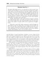
is called visual fit because one simply draws a straight line through the data
that “best fits” the pattern (see Exhibit 3.13). The point where this line inter-
sects the y-axis yields an estimate of the fixed cost component—those costs
that exist even without any sales activity. The slope of the line drawn is de-
fined mathematically as: rise over run or change in y-axis values divided by the
change in x-axis values. Using business rather than mathematical terminology,
how much the total costs change (the y-axis or rise) as the sales volume changes
(the x-axis or run). As was discussed above, this is simply the variable cost ex-
pressed as a percentage of sales. For the Books “R” Us example, given the line
I’ve drawn subjectively, the result would be:
With today’s computer software, this method is easy and time efficient. Unfor-
tunately, it lacks verifiability. If 20 people were to analyze this same data set,
you could end up with twenty different cost structure estimates.
The second method is called high-low analysis. It also is time efficient
and has the added advantage of verifiability. Since it is rule based, all twenty
people in this case would arrive at the same estimate. It has four steps:
1. On the x-axis, identify the high and the low points of the data set.
2. Identify the historical costs for each of those points.
3. Assume a straight line through these two points and calculate the variable
cost component using the traditional slope equation:
4. For either the high or the low set of data points, plug the values into the
cost equation and solve for the fixed cost component.
Slope
Change in - xis Values
Change in - xis Values
=
yA
xA
Fixed Cost Estimate: line crosses -axis at about million dollars
Variable Cost Percentage of Sales Estimate Slope: about 85.2%

9
y $4
=
EXHIBIT 3.13 Books “R” Us scatter plot.
0 5,000 10,000 15,000 20,000 25,000
Revenue ($)
Total Cost ($)
0
5,000
10,000
15,000
20,000
25,000
30,000
Cost-Volume-Profit Analysis 119
For the example and data set in Exhibit 3.12, the steps would be as
follows:
1. High and low points = September sales or $23.75 million and July sales of
$11.5 million.
2. Historical costs for each point = $25,000 (September) and $13,000 (July).
3. Slope = Rise/Run = ($25,000 − 13,000)/($23,750 − $11,500) = 98%.
4. Fixed component: Total Cost = Variable Cost + Fixed Cost.
For high data points:
For low data points:
This method has two weaknesses. First, the high and low data points chosen
are assumed to reflect the pattern of all data points. Often, however, either or
both of these points may not be such, and the analysis is flawed.
10
The second
weakness is an extension of the first. We had 12 data points but chose to ana-

lyze only two of them, ignoring the other 10. This method is data inefficient; if
you have 12 data points, all 12 should be considered for the analysis.
The third databased technique is called regression analysis. Here a func-
tion is fit through all data points in a manner that minimizes the total squared
error between each data point and the fitted line. The mathematics underlying
this technique are beyond the scope of this chapter, but the method is widely
used and preferred when the data set has problems such as a stepped fixed cost
or variable costs based on multiple factors. All spreadsheet software packages
have a function that performs simple regression analysis.
11
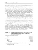
Exhibit 3.14 is an
example of what the output would look like for a least-squares regression analy-
sis using Excel. The estimate for the fixed cost is $2.73 million, and the vari-
able cost is 90% per sales dollar. The adjusted R
2
of 98% means that 98% of
the variance of the Total Cost data is explained by this equation. The drawback
of this analysis is that it is not intuitive. One must trust the output from the sta-
tistical package. If the user does not understand the statistical technique and
the assumptions of the software package, the output is often flawed.
12
This ap-
proach needs a sound grounding in statistical analysis.
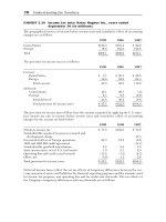
In summary, for the data set being analyzed, the three databased tech-
niques yield results that vary considerably (see Exhibit 3.15). The key to
correctly using databased techniques, however, is not choosing the right tech-
nique but beginning with a data set that truly reflects the cost structure being
$, %($, )
$, %($, )
$.

13 000 98 11 500
13 000 98 11 500
1 725
=+
=−
=
Fixed Cost
Fixed Cost
million (rounded)
$, %($, )
$, %($, )
$.
25 000 98 23 750
25 000 98 23 750
1 725
=+
=−
=
Fixed Cost
Fixed Cost
million (rounded)
120 Understanding the Numbers
analyzed. To emphasize this, the cost function, Total Cost = (76%)Revenue
+ $5 million, was used to generate the data set in Exhibit 3.12. A randomized
error term was then added to these data estimates, they were rounded to the
nearest quarter million, and then the high and low data points, July and Sep-
tember, were purposely changed. For instance, assume September was a very
busy month for Books “ ” Us because of the many college-student book or-
ders. This rush caused overtime and other disruptive cost behavior. Without
the analyst first adjusting the data point for this aberrant behavior, the results

are skewed. For databased techniques such as these, the adage “Garbage in,
garbage out” holds true. Before employing any of these techniques first ensure
that your data does truly reflect the cost structure being studied.
R
EXHIBIT 3.14 Least-squares regression output (Books “R” Us data).
SUMMARY OUTPUT
Regression Statistics
Multiple R 99.1%
R square 98.2%
Adjusted
R square 98.0%
Standard
error 471.36
Observations 12
ANOVA
df SS MS F Significance F
Regression 1 119,835,495 119835495 539.363 4.956E-10
Residual 10 2,221,797 222179.69
Total 11 122,057,292
Coefficients
Intercept $2,733
X variable 1 90%
EXHIBIT 3.15 Databased cost structure estimates.
Variable Cost Fixed Cost
Percentage (in millions)
Visual fit 85 $4.0
High-low 98 1.725
Least squares 90 2.733
Cost-Volume-Profit Analysis 121
THE ROLE OF PRICING IN CVP ANALYSIS

CVP analysis is often erroneously used to set prices. The P in CVP does not
stand for “price”; it stands for “profit.” A rule to remember: There is no such
thing as “cost-based pricing.” Prices are market driven. If a firm finds itself in
a competitive market where competition among rivals is based on delivering
comparable value to customers at the lowest cost, the market sets the price. As
Adam Smith wrote centuries ago, only the most efficient firms will survive. To
use CVP analysis in this situation, one starts with estimates of the market-
driven price and then calculates the profitability given probable unit demand
and the current cost structure. If the forecasted profit is not sufficient to sat-
isfy investors, one must then focus on reducing costs, not raising prices.
Incumbent firm behavior in the U.S. health care industry after deregula-
tion in the 1980s is a perfect example of incorrect use of this technique. New
entrants into the lower, more profitable segments of this industry—for exam-
ple, the walk-in clinics that have sprung up in metropolitan areas—gave pa-
tients (and insurance providers) a lower-cost option than traditional hospitals
for minor health-care procedures. Large hospitals responded to this loss of seg-
ment revenue by spreading their costs (mostly fixed) over their remaining
health-care offerings and raising prices. With those higher prices, the clinics
were able to offer lower-priced alternatives for more complex procedures.
With the loss of these revenues, the hospitals responded in the same manner.
This is called the “doom loop,” and it led to the closing of many such institu-
tions. The proper move for the hospitals should have been to pare expenses on
the noncompetitive offerings.
For firms that compete by differentiating themselves from rivals by offer-
ing additional value to customers at comparable cost, pricing should be based
on value to the customer, not cost. Microsoft certainly does not price its prod-
ucts on the costs to develop and deliver them. Bill Gates long ago understood
the value of an industry-standard PC operating system and has priced Micro-
soft’s offerings accordingly. The key here, of course, is that the additional value
must exceed the costs to create it. CVP analysis in this situation is basically no

different than previous examples. Only here, one starts with estimates of the
value-based price and then calculates the profitability given probable unit de-
mand and the current cost structure. If the forecasted profit is not sufficient to
satisfy investors, one must then focus not simply on raising prices but on reduc-
ing costs or increasing the willingness of consumers to pay more.
Predatory Pricing
In recent years a legal battle raged between two of the nation’s largest tobacco
companies.
13
The Brooke Group Inc. (previously known as Liggett Group Inc.)
accused Brown & Williamson Tobacco Corporation of predatory pricing in the
wholesale cigarette market. At trial in federal court the jury decided that
Brown & Williamson had indeed engaged in predatory pricing against Brooke.
122 Understanding the Numbers
The jury awarded damages of $150 million to be paid to Brooke by Brown &
Williamson. However, the presiding judge threw out this verdict. Brooke then
filed an appeal, and the case continued.
Predatory pricing cases are not unusual, and damage awards as large as
$150 million are not unheard of. Predatory pricing, as the name implies, is a
tactic where the predator company slashes prices in order to force its competi-
tors to follow suit. The purpose is to wage a price war and inflict upon the
competition losses of such severity that they will be driven out of business.
After destroying the competition, the predator company will be free to raise
prices so that it can recover the losses it sustained in the price war and also
rake in profits that will greatly exceed normal earnings at the competitive
level. This final result is harmful to competition, and predatory pricing has
therefore been made unlawful.
To determine whether a firm has engaged in predatory pricing, the courts
need a test that will supply the correct answer. One of the usual tests is
whether there is a sustained pattern of pricing below average variable cost. If

the answer is yes, this indicates predatory pricing. Let us examine the logic un-
derlying this widely used test.
First, recall that contribution is the margin between selling price and
variable cost. Contribution goes toward paying fixed costs and providing a
profit. If price is less than variable cost, contribution is negative. In that case,
the firm cannot fully cover its fixed costs, and certainly it will suffer losses.
Therefore, it makes no sense for the firm to charge a price that is below vari-
able cost unless the firm is engaging in predatory pricing in order to destroy
competing firms. That is why pricing below variable cost is considered to be
consistent with predatory pricing.
We should bear in mind that the variable cost used in the test is that of
the alleged predator, not of the alleged victim. The reason is that the alleged
predator may be an efficient low-cost producer, whereas the alleged victim
may be an inefficient high-cost producer. Therefore, a price below the alleged
victim’s variable cost may be above that of the alleged predator, in which case
it could be a legitimate price and simply a reflection of the superior efficiency
of the alleged predator. The antitrust laws are designed to protect competition,
but not competitors (especially those competitors who are inefficient).
Of course, this is only one indicator of predatory pricing, and all of the
relevant evidence must be considered. There should also be a pattern of sus-
tained pricing below variable cost. Prices that are slashed only sporadically or
occasionally are probably legitimate business tactics, such as loss-leader pricing
to attract customers or clearance sales to get rid of obsolete goods.
Predatory pricing is an important topic and has been the subject of major
lawsuits in a wide variety of industries. Because it is a common test for preda-
tory pricing, variable cost is also a very important topic that all successful busi-
nesspeople will benefit from thoroughly understanding.
Predatory pricing is usually thought of in a regional sense, or perhaps on a
national scale. But it can also occur on an international basis. In that case, it is
known as dumping.

Cost-Volume-Profit Analysis 123
Dumping
If a foreign company is the predator, there is no inherent difference in the tac-
tics or the goal of predatory pricing. Pricing below variable cost would still re-
main a valid test. However, U.S. law imposes a stricter test on foreign than on
domestic companies. The legal test for dumping does not involve variable cost.
Rather, it focuses on whether the foreign company is selling its product here at
a price less than the price in its home market.
Dumping is simply predatory pricing by a foreign company. So the logic
that supported using variable cost as a test for predatory pricing would also
support using the same test for dumping. But the test actually used is the
domestic selling price (usually higher than variable cost). This test makes it
easier to prove dumping than to prove predatory pricing. It favors the domestic
firms and is harder on the foreign company. This may be a matter of politics as
well as one of economics.
Perhaps the best-known cases of dumping have involved the textile and
steel industries. Another recent case of dumping concerned Japanese auto
companies accused by U.S. competitors of dumping minivans in this country.
Also, the Japanese makers of flat screens for laptop computers (active matrix
liquid crystal displays) were alleged to have sold their products in the United
States at prices below those in the home market.
It is not always easy to ascertain the home market selling price. Even if
there are list prices or catalog prices in the home market, there may be dis-
counts or rebates that are difficult to detect. Therefore, instead of using the
home market selling price as the test, the production cost may be used instead.
This is reasonable, because the production cost is likely to be below the home
market selling price. Therefore a dumping price below production cost is vir-
tually certain to be also below the home market selling price. But production
cost includes both fixed and variable costs and is therefore above variable cost.
Also, it may be arguable as to what should be included in production cost. For

example, some may include interest expense on money borrowed to purchase
manufacturing material inventories. Others may believe that interest is not
part of production cost.
If it is determined that dumping has indeed taken place, then the U.S. In-
ternational Trade Commission (ITC) will impose an import duty on the foreign
product involved. This duty will be sufficiently high to boost the U.S. selling
price to the same level as the home market price.
Dumping has a large potential impact on businesses and industries in our
economy. By extension, production cost is also a subject that successful busi-
nesspeople will find profitable to understand.
FOR FURTHER READING
Garrison, Ray, and Eric Noreen, Managerial Accounting, 8th ed. (New York: McGraw-
Hill, 1999).
Hilton, Ronald, Managerial Accounting, 4th ed. (New York: McGraw-Hill, 1998).
124 Understanding the Numbers
Horngren, Charles, Cost Accounting: A Managerial Emphasis, 9th ed. (Upper Saddle
River, NJ: Prentice-Hall, 1998).
Zimmerman, Jerold, Accounting for Decision Making and Control, 3rd ed. (New York:
McGraw-Hill, 1999).
NOTES
1. Mixed simply means that it has both a variable- and a fixed-cost component.
Mixed costs are very common—note your monthly phone bill or many car rental
contracts.
2. Economists argue that variable costs should not be represented by linear
functions, since economies and diseconomies of scale do exist. For instance, price
discounts are often given if one buys inputs such as paper for book printing in large
quantities. They are better represented by quadratic functions. Most agree, however,
that if we are analyzing a narrow enough range the assumption of linearity does not
lead to material error.
3. This can be expressed in an algebraic equation as follows. Since the indiffer-

ence point is where the two alternatives are equal:
Solving for x yields:
4. Defining the parameters of a “short-run” decision is often difficult. For this
special offer, if accepted, will PBS assume that this will be the price in the future?
Will other customers learn of this offer and expect the same terms? Short-run deci-
sions often have hidden long-run effects—they should always be scrutinized.
5. In this format, x represents required dollar sales volume, not required unit
sales volume.
6. ABC analysis, which is covered in the following chapter, is one such
technique.
7. When estimating cost structure from historical data the analyst must first
ascertain that the structure has not changed during the period being analyzed. If
Books “ ” Us made major additions to its infrastructure, it would make little sense to
aggregate the costs pre- and postaddition and consider them to be representative of a
single cost structure.
8. For this simple example we will assume that there are none of the seasonali-
ties in the fixed cost one would expect, say, for heating costs during the winter in New
England. Likewise, we will assume that the variable cost per dollar of revenue is the
same for all types of books.
R
$$,
$,
$
,
11 100 000
100 000
11
9 091
x
x

=
=
= units
$$$,12 23 100 000xx=−
Cost-Volume-Profit Analysis 125
9. To compute the slope, find a point that the line intersects and then measure
the “rise-over-run” using the y-axis intercept and that point. For this calculation my
line intersected the June data at point ($13,500, $15,500) so my rise was $11,500
($4,000 to $15,500 in Total Cost) and my run was $13,500 ($0 to $13,500 in Revenue).
The slope, therefore, was $11,500/$13,500 or 85.2%.
10. To avoid this shortcoming, many analysts first plot the data and then select
high and low data points that “best fit” the data set. This technique is a melding of
the first two databased techniques discussed.
11. For instance, Excel has a function that will perform a simple least-squares
regression on a given data set. Other regression techniques that relax the linear fit as-
sumption are also available on many statistical software packages.
12. For instance, infrastructure may have been expanded over the period
the data set covers. The regression software will assume a constant fixed cost rather
than some type of step function unless otherwise told. This can be treated using
dummy variables, but the user needs to have a working knowledge of the statistical
technique.
13. The final two sections of this chapter were written by John Leslie Living-
stone for earlier editions of this book. They are reproduced here in their entirety.
126
4
ACTIVITY-BASED
COSTING
William C. Lawler
Dave Roger, CEO of Electronic Transaction Network (ETN/ W), sat stunned
in his office. He had just come out of a preliminary third-round financing

meeting with potential investors. Six months ago his CFO had assured him that
third-round financing would not be a problem. Much had happened since that
date. The Internet stocks had crashed. Money for the technology sector was
now tight. In the two rounds before the crash, ETN/ W had so many prospec-
tive investors, the company had to turn some away. Since then their business
model had not changed; ETN/ W had a solid revenue stream, and the forecast
was for continued revenue growth—unlike many of the recently failed Inter-
net companies, ETN/W had real customers who were happy with its services.
Yet the meeting had concluded without closure on the third round for one sim-
ple reason. When Dave started talking about their “proven” business model the
potential investors immediately asked for specific details—“Explain your busi-
ness model in terms of how you will create wealth for us, your investors.”
As he fumbled to explain how ETN/ W would create shareholder wealth,
they stopped him and suggested an approach with which they were all
comfortable.
If you were a manufacturer we would expect you to tell us how you will use our
investment—some goes to infrastructure such as plant and equipment and some
to working capital such as inventory and receivables. You would then tell us how
much it would cost you to build your product, how much to market it, how much
to service it, and what customers would be willing to pay for it. Our first two
rounds of investment would have given you sufficient experience to gather this
type of data. With this information, you could explain your business model—
how you would create enough wealth to pay back our principal plus our required
Activity-Based Costing 127
return. Now, since you are a service provider rather than a manufacturer, ex-
plain your business model in like terms. What infrastructure is necessary for
your business? What does it cost you to provide your service? How much does it
cost to market these services? What are customers willing to pay for it?
As he sat there now, Dave wondered if the analogy the investors had used
was appropriate. In a manufacturing environment these questions were more

easily answered than in a service company like ETN/W. Yet after two rounds of
investment and eighteen months in business he had fumbled the most impor-
tant question in the meeting. In his hand he had the business card of a con-
sultant suggested by his investors. They said this person had worked with a
number of their clients and could help him develop the appropriate analysis. As
much as he disliked being pushed by anyone to make decisions, he knew that 25
employees were counting on him. He lifted the phone to call Denise Pizzi.
PR EPARING FOR DENISE
Denise was very professional on the phone. She was awaiting his call and sug-
gested that he prepare some documentation for their first meeting: a brief his-
tory of the company, their customer value proposition (she called it CVP), a
blueprint of the value system for their industry, and their strategy—what was
it that ETN/ W could offer clients that was distinct and value producing? Much
of this had already been prepared.
ETN/W History
Three MBA classmates with extensive experience in electronic commerce had
founded ETN/ W in Dallas, Texas, 18 months ago. Two came from a Houston
computer giant—Carol Kelly from the hardware side and Eric Rock, a senior
software applications manager. The third, Dave Roger, came from a well-known
Dallas IT consultancy, a company focused on the Internet and e-commerce.
The
idea had come from Dave. Many of his clients were in e-commerce, and all had
the same problem—transaction processing. Although most people think on-
line commerce is a relatively simple process—point and click—it is actually
quite complicated (see Exhibit 4.1). Assume customer A buys an item
at Books “ ” Us. When the order comes in, the company must first ascertain
A’s creditworthiness. This means a credit check with a payment processor. If
credit is okay, then Books “ ” Us has to contact the book wholesaler it partners
with to see if the book is in stock (this is called fulfillment). If the answer is in
the affirmative, Books “ ” Us gives the wholesaler the appropriate shipping

information, gets the tracking information from the shipper, and contacts the
payment processor once more to charge customer A. Books “ ” Us then relays
this information to A. This all has to be done in real time. Customer A does not
want to wait and will quickly move to a competitor if not satisfied. In addition,
R
R
R
R