Process Selection - From Design to Manufacture Episode 2 Part 7 potx

//SYS21///INTEGRAS/B&H/PRS/FINALS_07-05-03/0750654376-CH003.3D – 284 – [249–300/52] 8.5.2003 8:58PM
These are material to process compatibility, geometry to process suitability, including com-
plexity, size and thickness, tolerance requirements and surface finish.
The equation used for the calculation of the relative cost coefficient, R
c
is as follows:
R
c
¼ C
mp
C
c
C
s
C
ft
½3:9
where C
mp
¼ relative cost associated with material-process compatibility when compared with
an ideal material process combination, C
c
¼ relative cost associated with producing different
geometries from the ideal for the process under consideration, C
s
¼ relative cost associated
with achieving a section reduction/thickness or size outside the envelope of the ideal design
and C
ft
¼ C
t

or C
f
(whichever is greater),
where C
t
¼ relative cost associated with obtaining a specified tolerance and C
f
¼ relative cost
associated with obtaining a specified surface finish.
The combination of C
t
and C
f
into C
ft
is based on the assumption that when a fine surface
finish is being produced, fine tolerances can be produced for the same amount of cost and vice
versa. Thi s method of comparison and accumulation of costs, based on the product of the
above variables, is analogous to the methodologies used by experts in the field of cost
engineering and cost estimating. Note that when engineering the above elements going to
make up R
c
(C
mp
, C
c
, C
s
, C
t

, and C
f
), they need to take account of all the secondary processing
required to achieve the specified reductions, tolerances and finish, etc. for the component
design. For a simple or ideal design of component each of the relative cost coefficients is unity,
but as a component design moves away from that state, the coefficients tend to increase in
magnitude thus increasing the processing cost.
If R
c
data is not obtained, any estimate produced will be a lower bound only, the quality of
the estimate will improve as more information is repres ented regarding the effect of the design-
dependent factors.
Addition of R
c
data for a new manufacturing process
The steps proposed are as follows:
1 Following on from the procedure for P
c
, select the process in the database nearest to the
new process to be added. Again, let us consider adding of reaction injection moldi ng to the
system. A similar process would be injection molding.
2 Examine the data used for the variable ‘C
mp
’ for the surrogate process and determine if this
can be used directly as it stands, if not decide by how much should it be changed. In the first
instance, this should be checked with sources including published material (manufacturing
books and manuals), manufacturing experts and sp ecialist suppliers. Obtain comparative
figures for the materials to be considered and tabulate the values.
3 Repeat process in (2) above for the determinat ion of the value for ‘C
c

’. Obtain comparative
figures against the respect ive shape categories and plot or tabulate the results. Refer to
shape classification charts.
4 Repeat process in (2) above for the value of ‘C
s
’. Obtain comparative figures taking account
of section reductions/thickness and size. Tabulate results.
5 Repeat process in (2) above for the value of ‘C
t
’. Obtain comparative figures taking account
of tolerance requirements. Tabulate results.
6 Repeat process in (2) above for the value of ‘C
f
’. Obtain comparative figures taking account
of finish requirements. Tabulate results.
284 Costing designs
//SYS21///INTEGRAS/B&H/PRS/FINALS_07-05-03/0750654376-CH003.3D – 285 – [249–300/52] 8.5.2003 8:58PM
7 Add the pilot data to the system and represent as such. Add reaction injection molding data
and make as pilot data only.
8 Check the data against known costs for compon ents well suited to the process and calibrate
accordingly. Calibrate new process to known case studies.
9 Add data to main database, coded as a new process. The user should be informed that cost
estimates are based on new data. Once the data is proven, code as a standard process.
3.3 Manual assembly costing
Many designs are created with complex assembly sequences and fitting an d handling opera-
tions involving complex and restricted motions, poor stability, difficult orientation and align-
ment and simultaneous multiple insertions. The overall effect is reduced assemblability
resulting in increased assembly times and cost. To improve the assemblability of a design,
each operation needs to be carefully considered. Since something like 50 per cent of all labor in
the mechanical and electrical industries is involved in assembly, fitting and handling processes

must be addressed in proactive DFA. The development of suitable insertion ports and
handling features is essential for cost-effective assembly operations. In the present DFA
methodologies, the fitting and handling analyses are used to evaluate insertion processes,
which are ranked quantitatively dep ending on the difficulty of the task. The higher the score
the more inefficient the assembly operation (fitting or handling) is assumed to be, with 1.5 as a
threshold value for unacceptable design of an individual operation.
Although the fitting and handling analyses are both well-established means of assessing
assembly operations, they are highly judgmental, require training in their application and have
no provision for design advice. Within a more proactive DFA methodology, such information
needs to be provided to the designer in a transparent and intuitive manner. The data should
enable the designer to consider the effects of component and assembly port design on the cost
of product assembly. The capability of individual handling and alignment features with
respect to their ability to help (or hinder) the assembly operation needs to be presented to
the designer.
In order to make progress it is intended to allow the designer to view the data at different
levels of detail, ranging from direct comparisons to detailed elements of specific features. The
use of different representations will be investigated to make the information user-friendly. One
way in which this may be possible is to take a more fundamental approach to the cost/time of
component fitting and to use graphical representations of the effects of design geometry to
allow for easy comparison at a glance, rather than sorting through tabulated data. In the
following, we shall consider manual assembly processes only. Manual assembly is by far the
most common assembly system used in industry, in spite of the advent of more dedicated,
automatic and programmable systems, mainly due to the inherent flexibility of manual or
human operations.
3.3.1 Assembly costing model
The total cost of man ual assembly comprises the sum of the total handling and fitting times
multiplied by the labor rate (includes tooling cost, equipment costs, direct labor, supervision
and overheads) in pence per second. The handling analysis below returns a Component
Handling Index, H, related to a time factor for handling. Similarly, the time associ ated with
the fitting of components in assemblies is represented by a Component Fitting Index,

Manual assembly costing 285
//SYS21///INTEGRAS/B&H/PRS/FINALS_07-05-03/0750654376-CH003.3D – 286 – [249–300/52] 8.5.2003 8:58PM
F, through a straightforward analysis of a component’s fitting characteristics. Therefore, the
total cost of manual assembly, C
ma
, is:
C
ma
¼ C
1
ðF þ HÞ½3:10
where H ¼ component handling index (seconds), F ¼ component fitting index (seconds) and
C
l
¼ labor rate (pence per second).
In order to calculate an assembly cost, two further assumptions must be made:
1 The ideal assembly time for a combined handling and fitting operation is between 2 and 3
seconds. The exact time is dependent on factors such as workplace layout, environment and
worker relaxation. In the case where an ideal time of 2 s is assumed, then the indices H and F
can be taken as values in seconds. If 3 s is assumed, it is necessary to multiply the indices by
1.5 to obtain an estimate for the assembly time in seconds.
2 The labor rate, C
l
, is calculated based on an annual salary of £15 000 (plus 40 per cent
overheads for a worker in the UK), for a 250 working day year (5 day week minus statutory
holidays), and a 7.5 h working day. This gives the cost of manual labor per second,
C
l
¼ 0.31 pence.
Component handling analysis

The component handling index, H, can be defined as:
H ¼ A
h
þ
X
n
i¼1
P
o
i
þ
X
n
i¼1
P
g
i
"#
½3:11
where A
h
is the basic handling index for an ideal design using a given handling process, P
o
is
the orientation penalty for the component design and P
g
is the general handling property
penalty.
Basic Component Handling Indices (A
h

) (select one only) The basic handling indices, A
h
,
for a selection of common component handling characteristics are shown in Figure 3.31.
Fig. 3.31 Basic handling index (
A
h
) for a selection of component handling characteristics.
286 Costing designs
//SYS21///INTEGRAS/B&H/PRS/FINALS_07-05-03/0750654376-CH003.3D – 287 – [249–300/52] 8.5.2003 8:58PM
We now go on to consider the determination of the design-dependent, time-related, penalty
indices associated with the geometry and characteristics of the design.
Orientation Penalties (P
o
) (select both from Figure 3.32)
General Handling Penalties (P
g
) (select as appropriate) The general handling indices, P
g
,
for a selection of common situations are shown in Figure 3.33.
Fig. 3.32 Orientation penalties (
P
o
).
Manual assembly costing 287
//SYS21///INTEGRAS/B&H/PRS/FINALS_07-05-03/0750654376-CH003.3D – 288 – [249–300/52] 8.5.2003 8:58PM
Component fitting analysis
The Fitting Index, F, for a particular process in the sequence of assembly is defined as:
F ¼ A

f
þ
X
n
i¼1
P
f
i
þ
X
n
i¼1
P
a
i
"#
½3:12
where A
f
is the basic fitting index for an ideal design using a given assembly process, P
f
is the
insertion penalty for the component design and P
a
is the penalty for additional assembly
processes on parts in place.
Basic Component Fitting Index (A
f
) (select one only) Fitting indices for a selection of
common processes is shown in Figure 3.34.

Fig. 3.33 Handling sensitivity index (
P
g
) for a selection of component handling sensitivities.
Fig. 3.34 Fitting indices (
A
f
) for a number of common assembly processes.
288 Costing designs
//SYS21///INTEGRAS/B&H/PRS/FINALS_07-05-03/0750654376-CH003.3D – 289 – [249–300/52] 8.5.2003 8:58PM
Fig. 3.35 (a) Component insertion penalties (
P
fi
).
Manual assembly costing 289
//SYS21///INTEGRAS/B&H/PRS/FINALS_07-05-03/0750654376-CH003.3D – 290 – [249–300/52] 8.5.2003 8:58PM
Fig. 3.35 (b) Component insertion penalties (
P
fi
)(contd).
290 Costing designs
//SYS21///INTEGRAS/B&H/PRS/FINALS_07-05-03/0750654376-CH003.3D – 291 – [249–300/52] 8.5.2003 8:58PM
We shall now go on to consider the determination of the design-dependent, time-related,
penalty indices associated with the geometry and characteristics of assembly port designs.
Insertion Penalties (P
f
) (select all from Figures 3.35 (a) and (b))
Additional Assembly Processes (P
a
) (select as appropriate) Figure 3.36 gives the additional

assembly process index, P
a
, or a number of assembly processes carried out on components
already positioned in the assembly build.
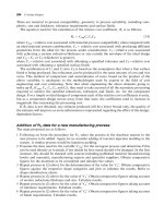
3.3.2 Assembly structure diagram
To facilitate a full assembly costing analysis, it is essential to understand the structure of the
proposed product, and an assembly structure diagram is useful in this respect. Through its use,
components in an assembly are logically mapped and in essence, represent the product’s
disassembly sequence from left to right. Constructing this diagram is seen as a beneficial
exercise, as it supports an assembly perspective upon the design and compels the designer to
focus on each component in the assembly. Included in the diagram are individual component
costs, M
i
, the manual assembly cost for each component, C
ma
, total M
i
and C
ma
for the
product and sub-assembly, and component identification labels. An example is shown in
Figure 3.37. Note that the inclusion of M
i
in the assembly structure diagram is optional.
A blank manual assembly costing table is provided in Appendix D to support the costing
methodology.
3.3.3 Manual assembly costing case studies
The design of a staple remover is shown in Figure 3.38. It is required to find the total
production cost of the staple remover, including the cost of manufacturing the components.
Figure 3.39 shows the assembly structure diagram for the assembled product, and the

assembly costing analysis to support the assembly cost figures for each ope ration is provided
in Figure 3.40. The component cost, M
i
, has already been determined from the methodology
provided earlier. The total cost of the stapler per unit is found to be approximately £0.23. Of
course, a profit margin (typically between 15 and 25 per cent) would be added to this cost, as
this is the cost to the company to manufacture and assemble the product. Packaging, shipping
and storage could also increase this cost substantially.
Fig. 3.36 Additional assembly index (
P
a
) for a number of common assembly processes.
Manual assembly costing 291
//SYS21///INTEGRAS/B&H/PRS/FINALS_07-05-03/0750654376-CH003.3D – 292 – [249–300/52] 8.5.2003 8:58PM
Figure 3.41 shows a possible redesign for the staple remover using just a single pressed sheet
metal component made from spring steel. Thi s design eliminates the need for any assembly
operations, although the cost of the material and complexity of the press tooling will only be
justified if a large volume is produced, in order to be competitive.
Fig. 3.37 Example format of an assembly structure diagram.
292 Costing designs
//SYS21///INTEGRAS/B&H/PRS/FINALS_07-05-03/0750654376-CH003.3D – 293 – [249–300/52] 8.5.2003 8:59PM
This second case study is concerned with just the assembly time and cost of a 1.44 Mb
floppy disk for use with a personal computer. Figure 3.42 shows the component parts. The
results are shown together with the assembly structure diagram in Figure 3.43, and a full
assembly costing analysis is provided in Figure 3.44. The total assembly cost of the floppy disk
per unit is found to be approximately £0.16, and the calculated assembly time is approximately
52 s. Note that a relaxation is not taken into account and the fact that the operator would be
working in a clean environment room wearing protective clothing to stop contamination.
The time contribution of each assembly operation compared to the overall assembly time is
shown as a percentage in Figure 3.45. A Pareto Chart format is used with the greatest contribu-

tion to the total assembly time to the left. As highlighted, locating the front case sub-assembly on
to the back case sub-assembly, whilst the spring is in position, is a difficult and time consuming
assembly task. Screen placement and spring fitting are two other operations of a time consuming
nature. In order to improve the assemblability of a particular concept design and reduce
assembly costs, the use of the metrics in this manner can help identify potentially problematic
areas and give guidance on redesign through reference to the charts provided.
3.4 Concluding remarks
The need to provide the concept design and development stages of the product introduction
process with carefully structured knowledge about process characteristics and capabilities,
together with cost estimating methods has been highlighted. PRIMAs of a standard form and
Fig. 3.38 Staple remover exploded view.
Concluding remarks 293
//SYS21///INTEGRAS/B&H/PRS/FINALS_07-05-03/0750654376-CH003.3D – 294 – [249–300/52] 8.5.2003 8:59PM
similar level of detail for each manufacturing process have been presented. Simple method s
based on economic and technical requirements have been designed to enable the user to focus
attention on the most relevant process quickly. The application of the data provided in the
PRIMAs as a means of selecting candidate processes has also been illustrated.
Fig. 3.39 Staple remover assembly structure.
294 Costing designs
//SYS21///INTEGRAS/B&H/PRS/FINALS_07-05-03/0750654376-CH003.3D – 295 – [249–300/52] 8.5.2003 8:59PM
Fig. 3.40 Staple remover assembly costing analysis.
Concluding remarks 295
//SYS21///INTEGRAS/B&H/PRS/FINALS_07-05-03/0750654376-CH003.3D – 296 – [249–300/52] 8.5.2003 8:59PM
A method for costing of designs, that can be used from concept to detail, has been
introduced. The novelty of the approach is the calculation of processing costs, based on the
notion of design-specific relative cost coefficients giving costs for processing idealized designs.
Results of validation trails have indicated that the cost analysis can be used to predict
component manufacturing costs, across a number of processes, to within 16 per cent of actual
values, using average process and material cost data. The performance of the analysis may be
much improved through the use of company specific data.

To support assembly-orientated design, it is essential to understand the cost implications of
the components designed on the assembly systems used. Various component features and
operations are known to exhibit higher assembly times than alternative combinations, and this
provides a basis for relatively comparing a number of concepts and calculating the assembly
time, and therefore the cost. The case studies have demonstrated the use of the methodology
for manual assembly.
The use of the PRIMAs and the costing analyses with DFA provides a more holistic means
of evaluating product designs and generating improved design solutions. In this way, the wider
application of DFA in industry is encouraged. In addition, the approach presented provides
for the carrying out of structured competitor analysis and yields a means for investigating
make versus buy decisions. There are opportunities for the development of computer software
to enhance the application of the process data and costing analysis. Potential benefits worth
noting in this connection include: removal of error prone manual calculation and reference to
maps and tables; consistency of results and standardized presentation; adherence to proce-
dure; time saving; ease of editing and ‘what if’ exploration; people’s operation and improved
version control.
Integration of computer-based process selection with other concurrent engineering software
tools, such as DFA, also offers potential benefits. The machine facilitates improved management
of information flow between the applications, and provides for common data entry, a
shared database, reuse and control of data and traceability of decisions. The CAD work-
station provides additional scope for the application and integration of simultaneous engin-
eering software tools within the design process. Design information from application of the
tools supplies useful input to the product modeling process.
Fig. 3.41 Staple remover redesign.
296 Costing designs
//SYS21///INTEGRAS/B&H/PRS/FINALS_07-05-03/0750654376-CH003.3D – 297 – [249–300/52] 8.5.2003 8:59PM
The development of new and advanced materials and the continuous search for improved
capability and lower processing costs means that process development is an important
research issue in manufacturing engineering circles. Consequently, the process selection
problem is something of a moving target. PRIMA development for standard processes is

not currently included, and catering for new processes as they emerge is an activity where
research effort is being placed. Also, feedback from users applying the work on new product
Fig. 3.42 Floppy disk component parts.
Concluding remarks 297
//SYS21///INTEGRAS/B&H/PRS/FINALS_07-05-03/0750654376-CH003.3D – 298 – [249–300/52] 8.5.2003 8:59PM
development projects, including views on what additional data they would like to see included
in the PRIMAs will provide a useful source of information for PRIMA development. Simi-
larly, user experience is being collected associated with application of the design costing
analysis. Investigating the employment of business specific data in place of that provided
for the sample set of processes included, and the incorporation by companies of data on
methods not in the set are other areas of research. In this way, much more will be understood
about ways of improving the analysis and its data, and the confidence that can be put on the
resulting cost estimates.
Before leaving the topic of design costing it is worth saying that when costing designs, the
costs of non-conformance must always be considered. There is little point in saving a few
pence or so on a component if attendant variability means rework, order exchange, warranty
claims, etc. The costs of failure can totally swamp any savings on manufacturing cost. The
intention behind the material presented here is to encourage the generation of capable design
solutions and facilitate the exploration of their likely cost implications. Selection must not be
based only on a minimum cost strategy. A ‘quality first’ strategy must be adopted.
Fig. 3.43 Assembly structure for a floppy disk.
298 Costing designs
//SYS21///INTEGRAS/B&H/PRS/FINALS_07-05-03/0750654376-CH003.3D – 299 – [249–300/52] 8.5.2003 8:59PM
Fig. 3.44 Floppy disk assembly costing analysis.
Concluding remarks 299
//SYS21///INTEGRAS/B&H/PRS/FINALS_07-05-03/0750654376-CH003.3D – 300 – [249–300/52] 8.5.2003 8:59PM
Fig. 3.45 Pareto chart of the assembly operation times for the floppy disk.
300 Costing designs
//SYS21///INTEGRAS/B&H/PRS/FINALS_07-05-03/0750654376-SAMPL.3D – 301 – [301–308/8] 8.5.2003 9:00PM
Sample questions for

students
The sample questions listed below provide some elemental ideas for examination questions and studies
for students of engineering and business.
1. In a business concerned with product design and manufacture, why is it worth giving considera-
tion to manufacturing process selection in the early stages of the design process?
2. What are the important criteria that influence process selection in a business? Consider both
technological and economic issues. State which of the criteria defined, set limits on what can be
achieved by the application of best practice in manufacturing operations.
3. Define a product introduction process and explain how it should be engineered to support the
creation of products that are economic to manufacture.
4. Why have businesses implemented formal product introduction process models and how do these
differ from the well-established design process models?
5. Present an outline classification of engineering materials indicating the main categories and their
subdivisions.
6. Define an outline classification of manufacturing processes indicating the main categories and their
subdivisions.
7. Where does process selection fit in a methodology concerned with design for manufacture and
assembly? Illustrate your answer with a simple flow chart.
8. Propose candidate material to process combinations for the following engineering components, and
justify any decisions made:
(a) Cylinder head for an internal combustion engine
(b) Spark plug body
(c) Radar dish
(d) 13 Amp power plug body.
9. Select three candidate methods for the manufacture of a low carbon steel tube, 20 mm diameter,
30 mm long with a uniform wall thickness of 2 mm. Rank each candidate for an annual production
quantity of 10 000.
10. Why are zinc alloys commonly used for the manufacture of die cast components and give some
typical examples?
11. The component shown in Figure Q.1 is to be manufactured by cold forming from a solid cylindrical

slug of cold forming steel. Describe the main steps involved in manufacturing the part and comment
on how the tooling would need to be proportioned to facilitate metal flow. Illustrate your answer
with a sketch.
12. A mezzanine floor is to be fabricated from 1 m square, 5 mm thick low carbon steel panels. Propose
methods for cutting the plate to size, preparing the edges, and welding the joints.
13. Compare injection molding and pressure die casting for the manufacture of a small lightly loaded
timer gear from a domestic appliance controller in terms of production rates and economics.
14. Contrast the manufacture of toothpaste tubes from aluminum and polymeric material.
//SYS21///INTEGRAS/B&H/PRS/FINALS_07-05-03/0750654376-SAMPL.3D – 302 – [301–308/8] 8.5.2003 9:00PM
15. Suggest suitable polymeric material and process combinations for the manufacture of the following
components, and justify any decisions made:
(a) Cylindrical bottle (1 l) for vegetable oil
(b) Automobile handbrake lever
(c) Computer casing
(d) Automobile bumper.
16. Compare the processing of metals and plastic by continuous extrusion and explain the differences
involved.
17. Contrast the application of adhesive bonding and spot welding for the assembly of pressed steel body
panels in automobile manufacture.
18. Suggest suitable composite or ceramic material and process combinations for the manufacture of the
following components, and justify any decisions made:
(a) Golf club heads and shafts
(b) Aeroplane propeller blades
(c) Metal cutting tool tips
(d) High performance hydraulic pistons.
19. In writing a guide for advising the designer regarding injection and compression molding, what
design rules would you include and why?
20. Contrast the manufacture of piercing and blanking press tool dies by conventional machining and
grinding, with electrical discharge machining.
21. Compare the production of machine tool stands or beds by fabrication techniques and sand casting

in terms of economic and technical considerations.
22. The component illustrated in Figure Q.2 is to be manufactured by injection molding unfilled
PBT. Given that dimension ‘A’ is a customer critical characteristic to be maintained at
Fig. Q.1 Cold formed plug body.
Fig. Q.2 Injection molded bush.
302 Sample questions for students
//SYS21///INTEGRAS/B&H/PRS/FINALS_07-05-03/0750654376-SAMPL.3D – 303 – [301–308/8] 8.5.2003 9:00PM
C
pk
¼ 1.33, estimate the cost of manufacture based on a production rate of 20 000 per annum.
(Answer: 8.3 pence)
23. Suggest suitable methods for joining the components in the following assemblies, and justify any
decisions made:
(a) A glass lens to the plastic molded automobile headlamp
(b) Alloy steel bicycle frame tube assembly
(c) Heavy duty chain links for lifting equipment
(d) Terminal posts and electronic components in printed circuit boards.
24. Compare the production of phosphor bronze plain bearings by machining and powder metallurgy in
terms of manufacturing economics and quality of conformance.
25. Contrast manually operated engine lathes, automatic lathes and CNC lathes in terms of manufac-
turing economics and technical capability.
26. The small aluminum alloy button shown in Figure Q.3 is currently produced by machining from
solid bar at an annual production quantity of 60 000. Would an annual cost saving be possible if the
part were to be made by pressure die casting?
(Answers: Machined ¼ 2.7 pence, Pressure die cast ¼ 3.1 pence)
27. Construct PRIMAs for the following processes:
(a) Stereolithography
(b) Water jet machining
(c) Flux cored arc welding
(d) Upset forging.

28. Collate and present component costing data that can be used with the costing analysis in Part III of
this book for the following manufacturing processes:
(a) Plaster mold casting
(b) Rotational molding
(c) Tungsten inert-gas welding
(d) Electrical discharge machining.
29. Explain how you would use the process capability charts presented with the PRIMAs in the
tolerancing of component assemblies, and in liaison with suppliers.
30. What are the main criteria that influence the cost of a manufactured component? State which of the
criteria are predetermined during the design process.
Fig. Q.3 Aluminium alloy button.
Sample questions for students 303